In general, the input to these problems includes a weighted set D of demand .... in the case of only five demand locations (|D| = 5), the problem cannot be solved using radicals; in particular, ... (4) A proof of NP-hardness for the k-median problem when the number of centers, ..... This is a constant expression, so f is cubic in x.
FACHBEREICH 3 MATHEMATIK
On the Continuous Weber and k-Median Problems (Extended Abstract)
by
´ndor P. Fekete Sa Joseph S. B. Mitchell Karin Weinbrecht No. 666/2000
On the Continuous Weber and k-Median Problems (Extended Abstract)
S´andor P. Fekete∗
Joseph S. B. Mitchell†
Karin Weinbrecht‡
Abstract We give the first exact algorithmic study of facility location problems that deal with finding a median for a continuum of demand points. In particular, we consider versions of the “continuous k-median (Weber) problem” where the goal is to select one or more center points that minimize the average distance to a set of points in a demand region. In such problems, the average is computed as an integral over the relevant region, versus the usual discrete sum of distances. The resulting facility location problems are inherently geometric, requiring analysis techniques of computational geometry. We provide polynomial-time algorithms for various versions of the L1 1-median (Weber) problem. We also consider the multiple-center version of the L1 k-median problem, which we prove is NP-hard for large k.
1
Introduction “There are three important factors that determine the value of real estate – location, location, and location.”
There has been considerable study of facility location problems in the field of combinatorial optimization. In general, the input to these problems includes a weighted set D of demand locations (with weight distribution δ and total weight A), a set F of feasible facility locations, and a distance function d that measures cost between a pair of locations. In one important class of questions, the problem is to determine one or more feasible median locations c ∈ F in order to minimize the average cost from the demand locations, p ∈ D, to the corresponding central points cp that are nearest to p: Z 1 δ(p)d (p, C) dp. min C⊂F A p∈D
If there is one median point to be placed, the problem is known as the classical Weber problem; it was first discussed in Weber’s 1909 book on the pure theory of location for industries [52] (see [54] for a modern survey). More generally, for a given number k ≥ 1 of facilities, the problem is known as the k-median problem. A problem of similar type with a different objective function is the so-called k-center problem, where the goal is to find a set of k center locations such that the maximum distance of the demand set from the nearest center location is minimized. With many practical motivations, geometric instances of facility location problems have attracted a major portion of the research to date. In these instances, the sets D of demand locations and F of feasible placements are modeled as points in some geometric space, typically 0 for all Z2 = (x2 , y2 ) with x2 > xm . Similarly, there is a unique horizontal median chord cy at y-coordinate ym . We call Zm = (xm , ym ) the L1 origin of P . In some situations, we make use of properties of higher-order derivatives of f . In particular, we use the following lemma: Lemma 4 Consider the objective function f for average straight-line or geodesic L1 distance in a region P . Let Z = (xz , yz ) be a point in P , with neither x nor y coinciding with the x- or y-coordinate of a local minimum or maximum of the boundary of P , and no point of the boundary of W (Z) or E(Z) coinciding with a vertex of P . Then there is a neighborhood of Z for which f is a cubic function in x and y. Proof. b1(t) B1 m1S m0N Z
0000000 1111111 0000000 1111111 00 11 0000000 1111111 00 11 0000000 1111111 00 11 0000000 1111111 11 00 0000000 1111111 0000000 1111111 0000000 1111111 0000000 1111111 0000000 1111111 0000000 1111111 0000000 1111111 0000000 1111111 0000000 1111111 0000000 1111111 0000000 1111111 0000000 1111111 0000000 1111111 0000000 1111111 0000000 1111111 0000000 1111111 0000000 1111111 0000000 1111111 0000000 1111111 0000000 1111111 0000000 1111111 0000000 1111111 0000000 1111111 0000 1111 0000000 1111111 0000 1111 0000000 1111111 0000 1111 0000000 1111111 0000 1111 0000000 1111111 0000 1111 0000000 1111111 0000 1111 0000000 1111111 0000 1111 0000000 1111111 0000 1111 0000000 1111111 0000 1111 1111 0000
h Z’
B0 11111 00000 00000 11111 00000 11111 00000 11111
00000 11111 00000 11111 00000 m0S b0(t)11111 00000 11111 00000 11111 00000 11111
11 00 00 11 00 11 00 11
m2N
00 11 11 00 00 11 00 11 00 11 00 11 00 11 00 11 00 11 00 11 00 11 00 11 00 11 00 11 00 11 00 11 00 11
y
000 111 00000 11111 000 111 11111 00000 000 111 00000 11111 000 111 00000 11111 000 111 000 111 000 111
B2 b2(t)
x
Figure 6: Trapezoids and slopes for higher order derivatives See Figure 6 for the case of straight-line distances, and consider changing Z to Z 0 = Z + (h, 0). Then W (x + h, y) = W (x, y) + B0 + B1 + . . . + Bk
(2)
E(x + h, y) = E(x, y) − B0 − B1 − . . . − Bk ,
(3)
and
7
with trapezoids B0 , . . . , Bk as shown in the figure. Let bi (t) be the width of trapezoid Bi at x-coordinate t, and miN and miS be the slopes of the upper and lower line segments bounding Bi . Then 1 Bi = hbi (x) + h2 (miN − miS ). 2 Then we get fxxx (x, y) = 2
k X
(miN − miS ).
i=0
This is a constant expression, so f is cubic in x. For geodesic distances, the claim follows in a similar manner. Instead of being trapezoids bounded by two vertical chords, however, the areas Bi are bounded by two bisectors of the SPM. It follows from elementary properties of L1 bisectors that these bisectors move in a parallel fashion, provided that during the move from Z to Z 0 , no polygon vertex is hit by the bisector. Thus, the Bi ’s are pseudo-trapezoids, and the area of each Bi is still a quadratic function of h. (Details are contained in the full version of the paper.) 2
4
Simple Polygons
In this section, we show how to compute in optimal (O(n)) time a point that minimizes the average geodesic L1 distance for a simple polygon. It follows from our observations from the previous section that a point has locally optimal x-coordinate if and only if its vertical chord passes through the L1 origin of the region. Let Zm = (xm , ym ) be this origin. In the following, we use the structure of simple polygons to show that Zm has to lie within the feasible region P . Theorem 5 The point Zm is feasible and thus a unique global optimum. Proof. Assume to the contrary that Zm is infeasible. Then the chord cx subdivides P into two or more pieces: let E denote the part to the right (“east”) of cx , and W the part to the left (“west”) of cx . Similarly, the chord cy subdivides P into two or more pieces, with N (“north”) denoting the part above cy , and S (“south”) denoting the part below cy . We distinguish the following cases, illustrated in Figure 7: Case 0: Neither cx nor cy are critical. If Zm 6∈ P , then, without loss of generality, the situation is as shown in Figure 7 (top). Then the two chords subdivide P into three pieces, E, W ∩ N , and S. By assumption, we have A(E) > 0, A(S) > 0, A(W ∩ N ) > 0, and A(E) + A(S) + A(W ∩ N ) = A(P ). Furthermore, the local optimality assumption on xm implies A(E) = 12 A(P ), and the local optimality assumption on ym implies A(S) = 12 A(P ). This implies A(W ∩ N ) = 0, a contradiction. Case 1: Precisely one of cx and cy is critical. If Zm 6∈ P then, without loss of generality, the situation is as shown in Figure 7 (center), with cy being critical. As in Case 0, the vertical chord cx partitions P into two pieces, “eastern” E and “western” W , and, by local optimality, A(E) = A(W ) = 12 A(P ). On the other hand, cy partitions P into an “upper” piece N , a “lower” piece S1 , and a second “lower” piece S2 , all with positive area. (Note that the interior of S2 may consist of several connected components, if the chord cy meets several local maxima of the boundary of P .) By local optimality, we know that A(N ) ≤ 12 A(P ), A(N ) + A(S2 ) ≥ 12 A(P ). Since N ∪ S2 ( E, we have a contradiction. Case 2: Both cx and cy are critical. If Zm 6∈ P then, without loss of generality, the situation is as shown in Figure 7 (bottom). As in Case 1, the horizontal chord cy subdivides P into a “northern” piece N , a “southern” piece S1 , and a second “southern” piece S2 , all with positive area. Similarly, the vertical chord cx subdivides P into a “western” piece W , an “eastern” piece E1 , and a second “eastern” piece E2 , all with positive area. By
8
y W
x
E
N
S
(Case 0)
N E
S2
W S1
(Case 1)
N S2
S1 W
E1
E2
(Case 2)
Figure 7: Intersection of median chords.
local optimality, we know that A(N ) ≤ 12 A(P ), A(N ) + A(S2 ) ≥ 12 A(P ), and similarly, A(W ) ≤ A(W ) + A(E2 ) ≥ 12 A(P ). Since N ∪ S2 ( E, we have a contradiction. 2
1 2 A(P ),
Theorem 6 The point Zm can be computed in linear time. Proof. We describe how to compute the x-coordinate xm of Zm ; the y-coordinate is found in a similar manner. In linear time (using Chazelle’s algorithm [10]), we build the vertical trapezoidization of P , which is defined by drawing vertical chords through every vertex of P . Each piece (cell), τi , of the map is either a vertical-walled trapezoid or a triangle (a degenerate trapezoid). Consider the adjacency graph G of these pieces τi (i.e., the planar dual of the trapezoidization); since P is a simple polygon, G is a tree. The x-coordinate xm of the optimal point Zm has to intersect some piece τm . Consider the partition of G induced by removing τm ; let Cmax be the heaviest connected component in this subdivision, and let τmax be the unique node of Cmax adjacent to τm . The weight of Cmax cannot exceed A(P )/2, or the local optimality of Zm would be violated: moving Zm from τm by an infinitesimal ε into τmax would reduce the distance to Zm by ε for a set of points of a total area more than A(P )/2, while increasing it by at most ε for a set of points of total area less than A(P )/2. Thus, τm is a median in the weighted tree G. 9
A median in a weighted tree can be computed in linear time (e.g., see Goldman [21]). This allows us to compute in linear time a piece τm that contains the critical coordinate xm . Once τm has been identified, it is easy to compute xm : assuming that xm is not given by one of the two vertical chords, we only have to identify the (unique) x-coordinate that splits P into two pieces of equal area. Since the slope of the boundary segments of τm does not change, this computation can be carried out by solving one quadratic equation. 2
5
Straight-Line L1 Distance
For straight-line distances, a finite average is guaranteed even for disconnected regions P , as long as they are compact. As in the case of geodesic distances, we can consider local optimality for finding a global optimum of f . The example in Figure 8 shows that even for the special case of a simple polygon P , the L1 origin of P may not be a feasible point.
P
Zm
Figure 8: For straight-line distances, the L1 origin of a simple polygon P may be infeasible This makes it more involved to compute all local optima. In the following, we describe how to evaluate them in O(n2 ) time. Theorem 7 For straight-line L1 distances, a point Z ∗ = (x∗ , y ∗ ) in a polygonal region P that minimizes the average distance f to all points in P can be found in time O(n2 ). Proof. We apply the local optimality conditions. We start by computing in time O(n log n) the L1 origin Zm of P ; if Zm is feasible (i.e., Zm ∈ P ), we are done. If no interior point of P is a local optimum, then we have to consider the boundary of P . This yields a set Ed of O(n) line segments and a set Vd of O(n) vertices that we examine for local optimality. We overlay the set of vertical and horizontal lines through all vertices of P with Ed , subdividing each segment in Ed into O(n) pieces, bounded by a total of O(n2 ) “overlay” vertices Vo . Let Eo be the resulting set of O(n2 ) subsegments. See Figure 9. Now we can examine the interior points pt = (t, y(t)) of each edge ej ∈ Eo for local optimality. Let sj be a vector parallel to ej . By construction of Eo , the vertical and horizontal lines through pt cannot encounter a vertex of P as pt slides along one subsegment of Eo . Thus, it follows from Lemma 4 that fx (pt ) is a quadratic function in t, then so is fy (pt ). Therefore, considering the local optimality condition h∇f, sj i = 0 for all O(n2 ) subsegments ej ∈ Eo yields a set of O(n2 ) quadratic equations in t. These can be solved in amortized time O(n2 ), since we can obtain the coefficients of each quadratic equation in amortized constant time by advancing from cell to cell in the overlay arrangement. This gives, for each subsegment ej , at most two local optima, qj,1 and qj,2 . Let V` be the union of Eo and all qj,1 and qj,2 . By construction, V` contains 10
y yn
y2 y1 x1
x2
xn x
x
Figure 9: Subdivision of the polygon into cells.
O(n2 ) elements, and all local optima of f occur at points of V` . Thus, our goal is to evaluate the objective function at each of these points and to select the best one. This is simply done in amortized time O(1) per candidate, by walking over the overlay arrangement and incrementally updating the value of the objective function. 2 In many cases, the following property of straight-line medians can be applied for a reduction of the set of boundary segment that we need to consider. (See Figure 10 for an illustration.) If Zm = (xm , ym ) is the L1 origin of P and p1 = (x1 , y1 ) and p2 = (x2 , y2 ) are points in P , we say that p1 dominates p2 , if p1 lies in the rectangle spanned by Zm and p2 . y p
2
p
1
Zm
x
Figure 10: p2 is dominated by p1 and cannot be a local optimum
Lemma 8 Let p1 = (x1 , y1 ) and p2 = (x2 , y2 ) be points in P . If p1 dominates p2 , then f (p1 ) ≤ f (p2 ). Proof. Suppose that x2 > x1 ≥ xm and y2 ≥ y1 ≥ ym . Then W (p2 ) ≥ W (p1 ) ≥ so moving a center from p2 to p1 cannot increase the objective value. 2
A 2
and S(p2 ) ≥ S(p1 ) ≥
A 2,
Using a plane-sweep algorithm, it is possible to identify the non-dominated pieces of the boundary in time O(n log n). If this set has complexity o(n), then we get a reduction of the overall complexity. An easy instance of the problem solved in this section is shown in Figure 11 (based on the simple example of Figure 1); this example shows the necessity of solving quadratic equations in computing the solution. We get the non-dominated points p1 , p2 , p3 and the edge e2,3 = p2 p3 .
11
x p
1
p
2
2x p4
- f(p4 ) p
(0,0)
5
p
3
√ √ Figure 11: The example from Figure 1 is analyzed: point p4 = (2 7 − 92 , 11 − 4 7) and its mirror image, p5 , are the two optima.
6
Geodesic Distances in Polygons with Holes
Now we discuss an even more complicated case, which arises when considering geodesic L1 distances in polygonal regions P that may have holes. Again, we analyze the set of locally optimal points: as long as a potential center can be moved in some axis-parallel fashion that lowers the average L1 geodesic distance to all the points, it cannot be optimal. The local optimality of a point Z is closely connected to the shortest path subdivision that it induces: for local optimality in the x-direction, the subdivision into W (Z) and E(Z) needs to be balanced; for local optimality in the y-direction, the subdivision into N (Z) and S(Z) needs to be balanced. The boundary between W (Z) and E(Z) is formed by bisectors for position Z. It follows from basic properties of shortest path maps that the total complexity of this boundary is O(n). (See, e.g., [40].) As we showed in Lemma 4, there is a neighborhood for each point Z ∈ P where the objective function f is cubic, provided that no bisector for Z meets a boundary vertex. This motivates the following lemma: Lemma 9 There is a subdivision of P of worst-case complexity I = Θ(n4 ), such that f is a cubic function within each piece of the subdivision. Proof. Lemma 4 implies that we are done if we can compute a subdivision of the claimed complexity such that we can move continuously between any two points in the interior of a connected cell of the subdivision, without any bisector encountering a vertex of the polygon during this motion. Provided that there is a position Z for which a bisector encounters a vertex v of the polygon, this vertex v is contained in W (Z) as well as in E(Z). Thus, there are two topologically different paths from Z to v, one fully contained in W (Z), the other contained in E(Z). This implies that there are two topologically different paths from v to Z, i. e., Z must lie on a bisector of v. Therefore, the required subdivision is obtained by considering the O(n) bisectors of the O(n) polygon vertices. Each bisector has a complexity of O(n), so the subdivision is defined by the overlay of O(n2 ) line segments, yielding an arrangement of worst-case complexity I = O(n4 ). Examples exist (see the full paper) to show that this bound on I is tight in the worst case. (Chiang and Mitchell [13] have studied similar arrangements that arise in overlaying shortest path maps in the Euclidean shortest path metric.) 2 Considering the local optima on each cell of the arrangement allows us to obtain the following: 12
Theorem 10 For geodesic L1 distances, a feasible point Z ∗ = (x∗ , y ∗ ) in a polygonal region P with holes that minimizes the average distance f to all points in P can be found in worst-case time O(I + n log n). Proof. (sketch) The idea is to reduce the problem to a set of O(I) candidates, with O(1) such candidates in the interior or on the boundary of each cell. The function parameters for f within each cell can be determined in total time O(I + n log n) by traversing the arrangement and doing updates when changing from one cell to its neighbor. After determining the O(I) candidate locations, we can determine a best among them by computing their objective values, again in total time O(I + n log n) by being careful how to update the objective function values. Thus, consider an arbitrary cell of the decomposition. If there is a local minimum interior to the cell, the gradient ∇f must vanish. Since f is cubic within the cell, this means that we get a system of two quadratic equations (both components of the gradient must be zero) with two variables (x and y). Such a system can be solved in constant time using radicals. Similarly, we can determine the local optima with respect to variation along a boundary segment of a cell. For each segment, the gradient needs to be orthogonal to the segment. As in the straight-line case, this yields a quadratic equation that can be solved in constant time. Finally, there are O(I) vertices in the arrangement, each of which we consider as candidates. 2
7
Many Centers
We now consider the k-median problem of placing k centers into a polygonal region P , such that the overall average distance of all points p ∈ P to their respective closest centers is minimized. We show that this problem is NP-hard for polygons with holes. Here, we give only an outline of the full proof. Our construction uses a reduction from Planar 3Sat. First, the planar graph corresponding to an instance I of Planar 3Sat is represented in the plane as a planar rectilinear layout, with each vertex corresponding to a horizontal line segment, and each edge corresponding to a vertical line segment that intersects precisely the line segments corresponding to the two incident vertices. There are well-known algorithms (e.g., [47]) that can achieve such a layout in linear time and linear space. See Figure 12. Next, the layout is modified such that the line segments corresponding to a vertex and all edges incident to it are replaced by a loop – see Figure 13 (top). At each vertex corresponding to a clause, three of these loops (corresponding to the respective literals) meet. Finally, the edges of all loops are replaced by a sequence of small squares that are interconnected by narrow corridors; also, each vertex for a clause is replaced by a single small square and linked to the adjacent variable loops by three narrow corridors. See Figure 13 (bottom) for the overall picture. Let 3k be the total number of squares in all variable loops. It can be checked that there is a placement of k variables with a low overall average distance of points to their closest centers (i.e., a low objective function value), if and only if there is a placement such that each square has a center or is next to a square with a center. This means that each clause square must be next to a square with a center. We prove that this is possible if and only if there is a satisfying truth assignment for the Planar 3Sat instance I. Details are contained in the full version of the paper.
8
Conclusions
In this paper, we have given the first exact algorithmic results for the Weber problem for a continuous set of demand locations. We have shown that for L1 distances in the plane, we can determine an optimum center in polynomial time, with the complexity ranging from O(n) for the case of geodesic distances in simple polygons, to O(n2 ) for straight-line distances in general polygonal regions, and O(n4 ) for geodesic distances in polygons with holes.
13
x1 C1 x2 C2 x3 C3 x4
C1 x1
x2 C3
C2 x3 x4
Figure 12: The graph GI for the Planar 3SAT instance I = (x1 ∨ x2 ∨ x3 ) ∧ (¯ x1 ∨ x ¯3 ∨ x4 ) ∧ (¯ x2 ∨ x3 ∨ x ¯4 ), and its geometric representation.
Our results rely on a careful understanding of the local optimality criteria. Our local optimality conditions generalize to the case of more general (non-uniform) nonnegative demand densities δ(p) by using the following observation. Regardless of the demand density function, any center location Z ∈ P induces a subdivision of P into E(Z) and W (Z), and N (Z) and S(Z) by shortest-path bisectors. Then the local optimality condition on Z requires that E(Z) and W (Z), and S(Z) and N (Z) are balanced in the following sense: instead of requiring thatR E(Z) and W (Z), Rand N (Z) and S(Z)R have the same area, R we consider the points Z where the integrals p∈W (Z) δ(p)dp and p∈E(Z) δ(p)dp, and p∈N (Z) δ(p)dp and p∈S(Z) δ(p)dp are the same. Points with these properties are called δ-medians. Similar ideas can be used for describing boundary points. If, for a particular δ, there is a limited number of δ-medians, they can be computed in polynomial time, and it is possible to compare objective values in polynomial time, then we can determine a δ-center for the given region. This includes the case in which the demand function is given by point weights in combination with a uniform demand distribution over P , which is a problem formulated by Wesolowsky and Love [55]. It is also easy to see that the above methods can be applied for the case in which F 6= D. Approximation algorithms for the Euclidean case can be devised based on generalizing the L1 metric results to fixed orientation metrics. The local optimality conditions become more complex; however, the inherent algebraic complexity remains the same, for any metric whose disks are convex polygons. Our methods can also be applied in higher dimensions, by generalizing the local optimality conditions and carrying through the analysis in a very similar manner to the two-dimensional case. Figure 14 shows that a generalization of Lemma 6, however, does not hold in three-dimensional space (the main reason being that any axis-parallel plane cuts the region into not more than two pieces), so we cannot use the same idea to exploit simplicity for achieving a better complexity than in the case with holes. However, we can still use a subdivision into cells and study the objective function within each cell. As in the two-dimensional case, the objective function is cubic for each coordinate, if P is a polyhedral region.
14
C1 x2
x1 C2
C3 x3
x4 C1
x1
x2 C3
C2
x3
x4
Figure 13: Replacing variables by loops (left); final polygon (right)
Figure 14: In three-dimensional space, there may not be a feasible point that is a median of P in all coordinates.
Acknowledgements We would like to thank Arie Tamir, Horst Hamacher, and Justo Puerto for pointing out relevant references and other helpful comments, Stefan Nickel for helpful comments, and Iris Weber for a heroic literature effort.
References [1] P. K. Agarwal, M. Sharir, and E. Welzl. The discrete 2-center problem. In Proc. 13th Annu. ACM Sympos. Comput. Geom., pages 147–155, 1997. [2] Y. P. Aneja and M. Parlar. Algorithms for Weber facility location in the presence of forbidden regions and/or barriers to travel. Transportation Science, 28(1):70–76, 1994. [3] C. Bajaj. The algebraic degree of geometric optimization problems. Discrete and Computational Geometry, 3:177–191, 1988. [4] R. Batta, A. Ghose, and U. S. Palekar. Locating facilities on the Manhattan metric with arbitrarily shaped barriers and convex forbidden regions. Transportation Science, 23(1):26–36, 1989. 15
[5] M. L. Brandeau and S. S. Chiu. An overview of representative problems in location research. Management Science, 35(6):645–674, 1989. [6] E. Carrizosa, M. Mu˜ noz-M´arquez, and J. Puerto. Location and shape of a rectangular facility in