On the correlation structures of multivariate skew-normal distribution

ACTA ET COMMENTATIONES UNIVERSITATIS TARTUENSIS DE MATHEMATICA Volume 20, Number 1, June 2016 Available online at http://acutm.math.ut.ee

On the correlation structures of multivariate skew-normal distribution ¨a ¨ rik, Meelis Ka ¨a ¨ rik, and Inger-Helen Maadik Ene Ka Abstract. Skew-normal distribution is an extension of the normal distribution where the symmetry of the normal distribution is distorted with an extra parameter. A multivariate skew-normal distribution has been parametrized differently to stress different aspects and constructions behind the distribution. There are several possible parametrizations available to define the skew-normal distribution. The current most common parametrization is through Ω and α, as an alternative, parametrization through Ω and δ can be used if straightforward relation to marginal distributions is of interest. The main problem with {Ω, δ}parametrization is that the vector δ cannot be chosen independently of Ω. This motivated us to investigate what are the possibilities of choosing δ under different correlation structures of Ω. We also show how the assumptions on structure of δ and Ω affect the asymmetry parameter α and correlation matrix R of corresponding skew-normal random variable.

1. Background We consider multivariate correlated data in broader sense including repeated measurements over time (longitudinal data) or space. To handle the dependence between measurements, it is essential to construct a full probability model that integrates the marginal distributions and the correlation coherently. For the multivariate normal distribution, such approach has been extensively investigated (see, for example, [23]). There are also many comprehensively examined analyses using simple correlation structure (uniform correlation and/or serial correlation). However, in many cases, the assumption of normality might be unrealistic, especially for skewed data. Data may be skewed naturally (consider, Received December 3, 2015. 2010 Mathematics Subject Classification. 60E15, 62H05, 60E05. Key words and phrases. Multivariate skew-normal distribution, compound symmetry correlation structure, autoregressive correlation structure. http://dx.doi.org/10.12697/ACUTM.2016.20.07 83

84

¨ ARIK, ¨ ¨ ARIK, ¨ ENE KA MEELIS KA AND INGER-HELEN MAADIK

e.g., the environmental pollution data in [11]) or because of conditioning while gathering the data (for example medical data of patients with certain diagnosis [13]). Conditioning causes a situation where (although the overall underlying distribution is normal) the gathered data actually follows a skew-normal distribution. The history of skew-normal distribution is not very long, but the development has been rapid and intensive. The first systematic representation of univariate skew-normal distribution is given by Azzalini [5]. The multivariate skew-normal distribution is introduced by Azzalini and Dalla Valle [10] and structured by Azzalini and Capitanio [7]. Extensions to the class are proposed by several authors [2, 8, 6, 16, 12]. Multivariate skew-normal distribution also has several different equivalent parametrizations, each of which offers advantages depending on a particular problem. To fully understand the mechanics of skewing, it is important to study the underlying dependence structures. A related widely studied example is the data of Australian athletes collected by Australian Institute of Sport (AIS-data). Various skewed models have been applied by different authors, main focus has been on the bivariate skew-normal distribution [10, 4, 3, 16] Similar problems in more general setup are addressed in [7], where a 5dimensional skew-normal model is applied to a diabetes data. ArellanoValle et al. developed a skew-normal mixed model for fitting longitudinal cholesterol levels data in Framingham heart study [1]. An extensive list of applications is given in [15, 6, 9]. Despite the growing number of publications, there remain several things to be explored. In this paper we examine the behaviour of the correlation matrices of multivariate skew-normal random variables in different specific situations starting from the more simple correlation structures like compound symmetry and autoregressive structure.

2. Framework The multivariate skew-normal distribution has received considerable attention over the last years. Nevertheless, even the “classical” multivariate skew-normal distribution, introduced by Azzalini and Dalla Valle in 1996, can be parametrized in many different ways starting from the initial {Ψ, λ}parametrization to the currently prevalent {Ω, α}-parametrization (see, e.g., [7], or, for a comprehensive analysis, [9]). Yet, because of the construction of α, the {Ω, α}-parametrization does not seem to be the most appropriate choice if the connection to the parameters of corresponding marginal distributions is of importance (see, e.g., [17, 19]). We have shown that the {Ω, δ}-parametrization is a reasonable choice, especially in the situation where direct connection with marginal parameters is of importance [20].

CORRELATION STRUCTURES OF MULTIVARIATE SKEW-NORMAL

85

We use {Ω, δ}-parametrization and analyze properties of the corresponding skew-normal random variable in different situations. We will reveal how the choice of correlation structure in Ω affects possible choices for δ and how the vector α is expressed in these special cases (recall that the vector α is determined by the vector δ and the concentration matrix Ω−1 ). The correlation matrix R and the region of possible correlation coefficients of the corresponding skew-normal random variable are studied as well. Let us first recall the definition of a multivariate skew-normal random variable through {Ω, δ}-parametrization. Definition 1. Let Ω be a positive definite k ×k correlation matrix and let δ be a k-dimensional vector such that δ T Ω−1 δ < 1. We say that a random variable Z = (Z1 , . . . , Zk )T has the k-variate skew-normal distribution with skewness parameter δ, and write Z ∼ SN (Ω, δ), if its probability density function is given by ! δ T Ω−1 z f (z; Ω, δ) = 2φk (z; Ω)Φ p , z ∈ Rk , (1) T −1 1−δ Ω δ where φk is the probability density function of the k-variate normal distribution with standard normal marginals and correlation matrix Ω, and Φ is the univariate standard normal distribution function. We also recall the following conditional representation of skew-normal variable (see, e.g., [10], [14] or [20] for {Ω, δ}-parametrization). If we have a k-dimensional random variable X ∼ N (0, Ω), a one-dimensional random variable X0 ∼ N (0, 1) and a vector δ = (δ1 , . . . , δk )T such that δ T Ω−1 δ < 1

(2)

and δ is the vector of correlations between X and X0 , then a random variable Z = X|X0 > 0 has the skew-normal distribution Z ∼ SN (Ω, δ). Considering the interpretation of δ as a vector of correlations it is useful to introduce the matrices ! ! 1 δT Ω δ ∗ Ω = , Ω∗ = , δ Ω δT 1 where Ω∗ is the correlation matrix for (X0 , X)T and Ω∗ is the correlation matrix for (X, X0 )T . In different applications, these matrices have important role and meaning. For example, in repeated measurement studies, the former has intuitive meaning if we consider conditioning by baseline and the latter in imputation of dropouts. In consequence, we have four correlation matrices related to a skew-normal random variable

86


• Ω = (ωij ) – the (scale) parameter matrix of the skew-normal distribution (see, e.g., (1)), • Ω∗ , Ω∗ – denoted above, • R = (rij ) – the correlation matrix of a skew-normal random variable Z, and it is now quite interesting to analyze the nature of restrictions on elements of these matrices. The general formula for computing the correlation matrix R = (rij ) of a skew-normal random variable Z = (Z1 , . . . , Zk ) is given by Azzalini and Dalla Valle [10] as follows: rij = corr(Zi , Zj ) = q

ωij − π2 δi δj , i, j = 1, . . . , k. q 1 − π2 δi2 1 − π2 δj2

(3)

An important special case is when all marginals have the same distribution SN (δ), that means all the components of δ are identical, i.e., δ = (δ, . . . , δ)T . Then the last formula simplifies to rij =

ωij − π2 δ 2 , i, j = 1, . . . , k. 1 − π2 δ 2

(4)

We are interested in structures of correlation matrices Ω, Ω∗ , Ω∗ , especially when they have the same stucture, and we would like to examine how their structure affects the structure of the correlation matrix R and the parameter vectors δ and α in different situations. A natural starting point is to use certain simple correlation structures depending on one parameter only. Thus, we consider the following correlation structures of Ω: (1) the exchangeable correlation structure or the compound symmetry (CS) when the correlations between all variables are equal, ωij = ω, i, j = 1, . . . , k, i 6= j; (2) the correlation structure, where the distance between variables in space or time determines the correlation (consider, e.g., autoregressive structure in repeated measurements or spatial processes). We focus on the simplest structure with this property: ωij = ω |j−i| , i, j = 1, . . . , k, i 6= j, and call this structure the autoregressive correlation structure (AR). Of course, there are various alternative structures for correlations available. We begin our analysis with the CS and AR correlation structures because of the distinctive reasons: they are the simplest most commonly used approaches and require the estimation of one parameter ω only, no matter how big the number of variables is.


87

3. Formulation of the problem Let us formulate the problem setup in more detail. Let Z = (Z1 , . . . , Zk )T have the k-variate skew-normal distribution, Z ∼ SN (Ω, δ), as specified in (1). Our aim is to investigate the effect of special cases of Ω to the corresponding skew-normal distribution. In the following we are going to study the aforementioned two special cases of Ω (CS, AR), starting with Ω = I as the simplest subcase of either structure. Two main special cases for vector δ are considered: (a) the case when all the components of parameter vector δ are identical, δ = (δ, . . . , δ)T , i.e., all marginals have the same distribution (i.e., SN (δ)); (b) the situation when the correlation matrix Ω∗ (or Ω∗ ) has also some simple structure. We search for answers to the following questions. (1) How can the parameter vector α of the corresponding {Ω, α}-parametrization be calculated? (2) What is the region of valid values for ωij (given δ)? (3) How can the correlation coefficients rij (defined in (3)) be calculated? (4) What is the region of possible correlation coefficients rij ?

4. The case when Ω = I and δ = (δ, . . . , δ)T Let us start with the simplest possible structure. Let Ω = I and δ = (δ, . . . , δ)T , i.e., the skew-normal distribution has i.i.d. marginals and the corresponding normal distribution has independent marginals. Let us recall the dual relation between the parameter vectors δ and α (see, e.g., [7]): Ω−1 δ (5) α= p 1 − δ T Ω−1 δ and Ωα δ=√ . (6) 1 + αT Ωα Taking into account our current assumptions, formulas (5) and (6) simplify to δ α α= √ , δ=√ . (7) 1 − kδ 2 1 + kα2 δ In other words, the vector α is in the form (α, . . . , α)T , where α = √ . 1 − kδ 2 The region of valid values for δ (with δ = (δ, . . . , δ)T ) also follows from (7): 1 1 δ ∈ −√ ; √ . (8) k k

88


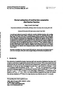
Also, Ω = I means that ωij = 0, i 6= j, which together with (4) implies 2δ 2 that rij = − , where rij = corr(Zi , Zj ) are the correlation coefficients π − 2δ 2 corresponding to the skew-normal random variable Z. The relationship between correlation coefficients rij = r and δ for some values of k is shown in Figure 1. k=30

r

−0.020

−0.010

−0.2 −0.4

r

0.0

0.000

k=2

−0.6

−0.2

0.2

0.6

−0.15 −0.05

delta

0.05

0.15

delta

Figure 1. Relationship between r and δ when Ω = I. We conclude that the correlation matrix of the random variable Z has the CS structure and, by (8), the region of possible values of correlation coefficients rij = r is given by 2 ;0 . (9) r∈ − kπ − 2 Remark 1. If the components of δ are identical, δ = (δ, . . . , δ)T , then the components of λ are also identical, λ = (λ, . . . , λ)T , and the following relations between δ and λ hold (see, for example, [10]): δ=√

λ ; 1 + λ2

λ= √

δ . 1 − δ2

Now, given Ω = I, the region of valid values for δ (8) also specifies the following region for valid values of λ: 1 1 λ ∈ −√ ;√ . k−1 k−1

5. The case when Ω has the CS structure Let us begin with a motivating example. Example 1 (Customer satisfaction data). The customer satisfaction index (CSI) is an economic indicator that measures the satisfaction of consumers. This is found by a customer satisfaction survey, which consists a questionnaire where the respondents (customers) are requested to give scores.


89

Now, for example, in case of benchmarking, we are interested in the behaviour of the customers whose score for specific questions is bigger (or smaller) than the overall mean or certain threshold. This implies that we have skewed data. Also, the whole customer satisfaction survey has usually several blocks of similar questions and the questions in blocks are correlated. The natural assumption is that the ordering of questions within a block does not matter, so we can assume the CS correlation structure. 5.1. The case when Ω has the CS structure and δ = (δ, . . . , δ)T . Let us assume that the correlation matrix Ω = (ωij ) has the CS correlation structure, i.e., ωij = ω, for i, j = 1, . . . , k, i 6= j. Consider the case of identical marginals, i.e., the vector δ has the form δ = (δ, . . . , δ)T . Formula (4) now simplifies to πω − 2δ 2 . (10) r= π − 2δ 2 In other words, the correlation matrix R also has the CS structure with parameter r. Now, from (10) it is easy to see that if δ is fixed, then r is a linear function of ω. (−1) To calculate α, let us first denote the elements of Ω−1 by ωij , i.e., (−1)

Ω−1 = (ωij (−1)

ωii

=

). Then the matrix Ω−1 has the following structure (see [21]):

1 + (k − 2)ω ω (−1) ; ωij = − , i 6= j. (1 + (k − 1)ω)(1 − ω) (1 + (k − 1)ω)(1 − ω)

Let us now apply formula (5) for α. The numerator Ω−1 δ is a k-dimensional vector with equal components (−1)

ωii

(−1)

δ + (k − 1)ωij

δ=

δ 1 + (k − 1)ω

and for the the denominator we get 1 − δ T Ω−1 δ =

1 + (k − 1)ω − kδ 2 . 1 + (k − 1)ω

In summary, the parameter vector α also has identical components, α = (α, . . . , α)T with δ p . α= p 1 + (k − 1)ω 1 + (k − 1)ω − kδ 2

(11)

Let us look what the restriction (2) implies on the correlation matrix Ω and on the correlation matrix R. Considering the positive definiteness of Ω and restriction (2) we get the following requirement for δ and ω: 0
0, the infimum of the rij is found in the process ω ↓ and by (23) we have

kδ 2 − 1 , (k − 2)δ 2 + 1


 rij ∈ 

2

kδ −1 |i−j| − 2δ 2 π( (k−2)δ 2 +1 )

π − 2δ 2

95

 ; 1 .

(24)

Exactly the same reasoning can be used if |i − j| is odd, thus the corresponding region of valid values for rij is also specified by (24). Remark 4. From a practical perspective, the situation where ω > 0 is obviously more common (consider, e.g., repeated measurements where the correlation decays in time). If ω > 0, then the region of valid values for rij becomes 2δ 2 ; 1 rij ∈ − π − 2δ 2 √ for both even and odd values of |i − j|, with |δ| < 1/ k, because of (22). This means that even if ω > 0, the rij can also have negative values. 6.2. The case when Ω and Ω∗ have the AR structures. Let us assume that Ω and Ω∗ have the AR structures. Note that if Ω∗ has the AR structure, then the vector δ is specified as follows: δ = (ω k , . . . , ω)T . Let us now derive a formula for corresponding α. We again start from the general relation (5) and calculate the numerator and denominator of given expression separately. For the numerator we get Ω−1 δ = (0, . . . , 0, ω)T , and the denominator therefore reduces to 1 − δ T Ω−1 δ = 1 − ω 2 . Also, as δ T Ω−1 δ > 0 if |ω| < 1, the region of valid values of ω is ω ∈ (−1; 1). Taking into account the forms of the numerator and the denominator of (5) under current assumptions, the components of α = (α1 , . . . , αk )T are ω . For the correlation the following: α1 = . . . = αk−1 = 0 and αk = √ 1 − ω2 coefficients we can see that the general formula (3) transforms to ω |i−j| − π2 ω 2k+2−i−j q rij = q . 2 2(k+1−i) 2 2(k+1−j) 1 − πω 1 − πω

(25)

The behaviour of rij for different choices of ω and k is shown in Figure 5. Remark 5. Let us now examine how the choice of ω affects the correlation coefficients rij . In the process ω ↑ 1 we have rij ↑ 1. In the process ω → 0 we have rij → 0 (the case of independent marginals). In the process ω ↓ −1, the value of rij depends on indices i and j: if |i − j| is even, then rij ↑ 1, and if |i − j| is odd, then rij ↓ −1. The dependence of the regions for valid values of rij from the parity of |i − j| is also illustrated in Figure 5. One can also see from this figure that bigger values of i and j produce smoother curve (especially if the difference


96

−0.5

0.0

0.5

1.0

0.8 r −1.0

−0.5

0.0

0.5

1.0

−1.0

0.0

0.5

omega

k=50, i=34, j=8

k=50, i=45, j=12

k=50, i=45, j=47

0.0

0.5

1.0

0.8 r 0.0

−1.0 −0.5

−1.0

−0.5

0.0

0.5

1.0

−1.0

−0.5

0.0

0.5

omega

k=500, i=338, j=340

k=500, i=416, j=411

k=500, i=37, j=67

0.0

0.5

1.0

0.8 r 0.0

−1.0

0.0

−0.5

−1.0

omega

1.0

0.4

r

r 0.4

0.0 0.5 1.0

omega

0.8

omega

−1.0

1.0

0.4

r

r 0.4

0.0 0.5 1.0

omega

0.0 −1.0

−0.5

omega

0.8

−1.0

0.0

0.0

−1.0

0.4

r

r 0.4

k=5, i=1, j=5

0.0 0.5 1.0

k=5, i=2, j=3

0.8

k=5, i=2, j=4

−0.5

0.0

0.5

1.0

omega

−1.0

−0.5

0.0

0.5

1.0

omega

Figure 5. The relationship between the correlation coefficients r and ω when Ω and Ω∗ have the AR structures. of i and j is small) and big difference between i and j results in rij = 0 except for the extreme cases when |ω| is close to 1. Although the correlation matrix R does not retain the AR-structure, it is worth noting that there still exists a certain structure. Proposition 1. Let Z follow a k-variate skew-normal distribution, Z ∼ SN (Ω, δ), such that Ω and Ω∗ have the AR structures. Then the correlation matrix R = (rij ) has the following property: j−1 i−1 Y Y rij = I{i