Journal of Computational Mathematics Vol.28, No.3, 2010, 386–400.
http://www.global-sci.org/jcm doi:10.4208/jcm.2009.10-m2636
ON THE FINITE ELEMENT APPROXIMATION OF SYSTEMS OF REACTION-DIFFUSION EQUATIONS BY p/hp METHODS* Christos Xenophontos Department of Mathematics & Statistics, University of Cyprus, P.O. BOX 20537, Nicosia 1678, Cyprus Email:
[email protected] Lisa Oberbroeckling Department of Mathematical Sciences, Loyola University Maryland, 4501 N. Charles Street, Baltimore, MD 21210, USA Email:
[email protected] Abstract We consider the approximation of systems of reaction-diffusion equations, with the finite element method. The highest derivative in each equation is multiplied by a parameter ε ∈ (0, 1], and as ε → 0 the solution of the system will contain boundary layers. We extend the analysis of the corresponding scalar problem from [Melenk, IMA J. Numer. Anal. 17(1997), pp. 577-601], to construct a finite element scheme which includes elements of size O(εp) near the boundary, where p is the degree of the approximating polynomials. We show that, under the assumption of analytic input data, the method yields exponential rates of convergence, independently of ε, when the error is measured in the energy norm associated with the problem. Numerical computations supporting the theory are also presented, which also show that the method yields robust exponential convergence rates when the error in the maximum norm is used. Mathematics subject classification: 65N30. Key words: Reaction-diffusion system, Boundary layers, hp finite element method.
1. Introduction The numerical solution of reaction-diffusion problems whose solution contains boundary layers has been studied extensively over the last two decades (see, e.g., the books [5, 6, 8] and the references therein). The presence of boundary layers in the solution cannot be overlooked, and if one wishes to obtain an accurate and robust approximation, special care must be taken when constructing the numerical method. In the context of the Finite Element Method (FEM), the robust approximation of boundary layers requires either the use of the h version on nonuniform meshes (such as the Shishkin [11] or Bakhvalov [1] mesh), or the use of the high order p and hp versions on specially designed (variable) meshes [10]. In both cases, the a-priori knowledge of the position of the layers is taken into account, and mesh-degree combinations can be chosen for which uniform error estimates can be established [2, 4, 10]. In recent years researchers have turned their attention to systems of reaction-diffusion problems — see [3] and the references therein for a recent survey. In general, one-dimensional reaction diffusion systems, like the one considered in the present article, have the following *
Received September 5, 2007 / Revised version received July 31, 2009 / Accepted August 25, 2009 / Published online February 1, 2010 /
387
On the FE Approximation of Reaction-Diffusion Equations by p/hp Methods
→ form: Find − u such that → L− u ≡
2
d −ε21 dx 2
0 ..
.
0 − → u (0)
=
− → → − u (1) = 0 ,
where 0 < ε1 ≤ ε2 ≤ ... ≤ εm ≤ 1, a11 (x) ... .. A= . am1 (x) ...
− → − → − → u +Au = f
in
Ω = (0, 1),
(1.1)
d2 −ε2m dx 2
(1.2) a1m (x) .. , . amm (x)
f1 (x) − → .. f (x) = . . fm (x)
(1.3)
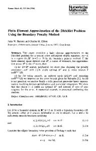
→ − m → The data {εi }i=1 , A and f are given, and the unknown solution is − u (x) = [u1 (x), ..., um (x)]T . The functions aij (x) are such that for any x ∈ Ω = [0, 1], the matrix A is invertible (with kA−1 k bounded) and moreover − →T − → → − − → → − ξ A ξ ≥ α2 ξ T ξ ∀ ξ ∈ Rm , (1.4) for some constant α > 0. We will restrict ourselves to the case εi = ε ∀ i = 1, ..., m, which allows us to express → (1.1)–(1.2) in vector form as: Find − u such that → − → → − L− u := −ε2 − u 00 + A→ u = f in Ω = (0, 1), (1.5) − → − → → − u (0) = u (1) = 0 . (1.6) The presence of the small parameter ε in the above boundary value problem causes the solution − → u to contain boundary layers of width O(|ε ln ε|) near the endpoints of Ω. To illustrate this, we consider the case m = 2 with · ¸ · ¸ − → 2 −1 2 A= , f (x) = , ε = 10−2 . −1 2 1 Figure 1.1 shows the exact solution corresponding to the above data and clearly shows that both components contain a boundary layer. Our goal in the present article is to extend the analysis of [4] for the analogous scalar problem, to show that under the assumption of analytic input data, the hp version of the FEM on the variable three element mesh ∆ = {0, κpε, 1 − κpε}, κ ∈ R+ converges at an exponential rate (in the energy norm defined in eq. (2.6) below) as the polynomial degree of the approximating basis functions p → ∞. Strictly speaking, the method is not an hp version, since the location and not the number of elements changes as the dimension of the approximating subspace is increased; a more appropriate characterization would be a p version on a variable mesh. In addition to extending the results of [4] to systems, our proof does not use Gauss-Lobatto interpolants (like the one in [4]), but rather we achieve the desired result using the approximation theory from [9] with integrated Legendre polynomials, something that is of interest in its own right. More importantly, the present approach allows us to define the constant κ used in the mesh in a more concrete way. The rest of the paper is organized as follows: In Section 2 we present the model problem and discuss the properties of its solution. In Section 3 we present the finite element formulation and the design of the p/hp scheme we will be considering, along with our main result of exponential
388
C. XENOPHONTOS AND L. OBERBROECKLING 1.8
1.6
1.4
1.2
1
0.8
0.6
0.4 u1(x) u2(x)
0.2
0
0
0.1
0.2
0.3
0.4
0.5 x
0.6
0.7
0.8
0.9
1
Fig. 1.1. The exact solution with ε = 10−2 .
convergence. In Section 4 we present the results of some numerical computations for two model problems, and in Section 5 we summarize our conclusions. In what follows, the space of squared integrable functions on an interval Ω ⊂ R will be denoted by L2 (Ω) , with associated inner product Z (u, v)Ω := u(x)v(x)dx. Ω
We will also utilize the usual Sobolev space notation H k (Ω) to denote the space of functions on Ω with 0, 1, 2, ..., k generalized derivatives in L2 (Ω) , equipped with norm and seminorm k·kk,Ω → and |·|k,Ω , respectively. For vector functions − u = [u1 (x), ..., um (x)]T , we will write 2 2 2 → k− u kk,Ω = ku1 kk,Ω + ... + kum kk,Ω .
We will also use the space
½ H01 (Ω) =
¾ u ∈ H 1 (Ω) : u|∂Ω = 0 ,
where ∂Ω denotes the boundary of Ω. Finally, the letter C will be used to denote a generic positive constant, independent of ε or any discretization parameters, and possibly having different values in each occurrence.
2. The Model Problem and its Regularity We assume that the functions aij (x) and fi (x) are analytic on Ω and that there exist constants Cf , γf , Ca , γa > 0 such that ° ° ° (n) ° ≤ Cf γfn n! ∀ n ∈ N0 , i = 1, ..., m, (2.1) °fi ° ° ° ° (n) ° °aij °
∞,Ω
∞,Ω
≤ Ca γan n! ∀ n ∈ N0 , i, j = 1, ..., m.
(2.2)
On the FE Approximation of Reaction-Diffusion Equations by p/hp Methods
389
As usual, we cast the problem (1.5)–(1.6) into an equivalent weak formulation, which reads: £ ¤m → Find − u ∈ H01 (Ω) such that £ ¤m → − → → B (− u,→ v ) = F (− v ), ∀ − v ∈ H01 (Ω) , (2.3) where → → B (− u,− v ) = ε2
m X
(u0i , vi0 )Ω +
i=1
→ F (− v)=
m X
m X m X
(aij uj , vi )Ω ,
(2.4)
i=1 j=1
(fi , vi )Ω .
(2.5)
i=1
From (1.4), we get that the bilinear form B (·, ·) is coercive with respect to the energy norm
i.e.,
2 2 2 → − → k− u kE,Ω := ε2 |→ u |1,Ω + α2 k− u k0,Ω ,
(2.6)
£ ¤m 2 → → → → B (− u,− u ) ≥ k− u kE,Ω ∀ − u ∈ H01 (Ω) .
(2.7)
This, along with the continuity of B (·, ·) and F (·) , imply the unique solvability of (2.3). We also have the a priori estimate →° 1° °− ° → k− u kE,Ω ≤ ° f ° . (2.8) α 0,Ω We now present results on the regularity of the solution to (1.5)–(1.6). Note that by the analyticity of aij and fi , we have that ui are analytic. Moreover, we have the following theorem, whose proof is a straight forward generalization of the proof of Theorem 1 from [4]. → Theorem 2.1. Let − u be the solution to (1.5)–(1.6) with 0 < ε ≤ 1. Then there exist positive constants C and K ≥ 1, independent of ε, such that ° ° ° (n) ° ≤ CK n max{n, ε−1 }n ∀ n ∈ N0 , i = 1, ..., m. (2.9) °ui ° 0,Ω
→ We will now obtain a decomposition for the solution − u into a smooth (asymptotic) part, two boundary layer parts and a remainder as follows: − → → − → → u =− w +→ u−+− u++− r.
(2.10)
This decomposition is obtained by inserting the formal ansatz − → u (x) ∼
∞ X
− εi → u i (x),
(2.11)
i=0
into the differential equation (1.5), and equating like powers of ε, so that we can define the → smooth part − w as M X → − → w (x) := ε2i − u 2i , (2.12) i=0
→ where the terms − u 2i are defined recursively by → − − → u 0 = A−1 f , 00 → − → u 2i = A−1 (− u 2i ) , i = 0, 2, 4, ...
(2.13) (2.14)
390 A calculation shows that
C. XENOPHONTOS AND L. OBERBROECKLING
00 → → → L(− u −− w ) = ε2M +2 (− u 2M ) ,
(2.15)
→ hence, as ε → 0, − w (x) defined by (2.12) satisfies the differential equation, but not the boundary → → conditions. To correct this we introduce boundary layer functions − u + and − u − by − → → − → → L− u − = 0 in Ω L− u + = 0 in Ω − → → u − (0) = −− w (0) − → − → u − (1) = 0 ;
→ − → − u + (0) = 0 → − → u + (1) = −− w (1).
(2.16)
→ Finally, we define − r by 00 − → L→ r = ε2M +2 (− u 2M ) , − → − → → r (0) = − r (1) = 0 .
(2.17a) (2.17b)
The following results follow from the analogous ones for the scalar problem considered in [4], and their puprose is to provide information on the regularity of each of the components in (2.10). → Lemma 2.1. Let − u 2i be defined as in (2.13)–(2.14). Then there exist positive constants → − C, K1 , K2 , (K2 > 1), depending only on A and f such that for any i, n ∈ N0 ° ° °→ (n) ° u 2i ) ° ≤ CK12i K2n (2i)!n!. °(− ∞,Ω
− → Theorem 2.2. There exist constants C, K 1 , K 2 ∈ R+ depending only on f and A such that − if 0 < 2M εK 1 ≤ 1, then → w (x) given by (2.12), satisfies ° ° n °→ ° (2.18) w (n) ° ≤ CK 2 n! ∀ n ∈ N0 . °− ∞,Ω
→ Theorem 2.3. Let − u ± be the solutions of (2.16). Then there exist constants α, C, K > 0 independent of ε and n such that for any x ∈ Ω, n ∈ N0 , and i = 1, ..., m, ¯¡ ¢ ¯ ¯ − (n) ¯ (x)¯ ≤ CK n e−xα/ε max{n, ε−1 }n , (2.19a) ¯ ui ¯¡ ¢ ¯ ¯ + (n) ¯ (x)¯ ≤ CK n e−(1−x)α/ε max{n, ε−1 }n . (2.19b) ¯ ui Theorem 2.4. There are constants C, K1 , K2 > 0 depending only on the input data such that → the remainder − r defined by (2.17b) satisfies ° ° °− ° 2M r (n) ° ≤ CK22 ε2−n (2M εK1 ) , n = 0, 1. (2.20) °→ 0,Ω
3. The Finite Element Method For the discretization of (2.3), we choose a finite dimensional subspace SN of H01 (Ω) and m → solve the problem: Find − u N ∈ [SN ] such that m → → → → B (− u ,− v ) = F (− v) ∀− v ∈ [S ] . (3.1) N
N
The unique solvability of the discrete problem (3.1) follows from (1.4) and (2.7); by the wellknown orthogonality relation, we have → → − → k− u −− u N kE ≤ → inf k→ u −− v kE . (3.2) − v ∈[SN ]m
On the FE Approximation of Reaction-Diffusion Equations by p/hp Methods
391
The subspace SN is chosen as follows: Let ∆ = {0 = x0 < x1 < ... < xM = 1} be an arbitrary partition of Ω = (0, 1) and set Ij = (xj−1 , xj ) , hj = xj − xj−1 , j = 1, ..., M. Also, define the master (or standard) element IST = (−1, 1), and note that it can be mapped onto the j th element Ij by the linear mapping x = Qj (t) =
1 1 (1 − t) xj−1 + (1 + t) xj . 2 2
With Πp (IST ) the space of polynomials of degree ≤ p on IST , we define our finite dimensional subspaces as © ª → − SN ≡ S p (∆) = u ∈ H01 (Ω) : u (Qj (t)) ∈ Πpj (IST ) , j = 1, ..., M , and
im h → − − →p S 0 (∆) := S p (∆) ∩ H01 (Ω) ,
(3.3)
→ where − p = (p1 , ..., pM ) is the vector of polynomial degrees assigned to the elements. The following approximation result from [9] will be the main tool for the analysis of the method. As mentioned earlier, the analysis for the scalar problem in [4] relied on Gauss-Lobatto interpolants (and their approximation properties), which is different from what we present in this work. ¡ ¢ Theorem 3.1. For any u ∈ C ∞ I ST there exists Ip u ∈ Πp (IST ) such that u (±1) = Ip u (±1) , ° 1 (p − s)! ° ° (s+1) °2 2 ku − Ip uk0,IST ≤ 2 , ∀ s = 0, 1, ..., p, °u ° p (p + s)! 0,IST ° ° ° (p − s)! ° ° (s+1) °2 °(u − Ip u)0 °2 ≤ u , ∀ s = 0, 1, ..., p. ° ° 0,IST (p + s)! 0,IST
(3.4) (3.5) (3.6)
The definition below describes the mesh used for the method: If we are in the asymptotic range of p, i.e. p ≥ 1/ε, then a single element suffices since p will be sufficiently large to give us exponential convergence without any refinement. If we are in the pre-asymptotic range, i.e. p < 1/ε, then the mesh consists of three elements as described below. We should point out that this is the minimal mesh-degree combination for attaining exponential convergence; obviously, refining within each element will retain the convergence rate but would require more degrees of freedom – one such example is the so-called geometrically graded mesh discussed in [4] for the scalar problem. − → Definition 3.1. For κ > 0, p ∈ N and 0 < ε ≤ 1, define the spaces S (κ, p) of piecewise polynomials by (− →p S 0 (∆); ∆ = {0, 1} if κpε ≥ 12 , − → S (κ, p) := − →p S 0 (∆); ∆ = {0, κpε, 1 − κpε, 1} if κpε < 21 . In both cases, the polynomial degree is uniformly p on all elements. Before we state the main theorem of the paper, we cite a useful computation.
392
C. XENOPHONTOS AND L. OBERBROECKLING
Lemma 3.1. Let p ∈ N, λ ∈ (0, 1]. Then " # (1−λ) p (p − λp)! (1 − λ) ≤ p−2λp e2λp+1 . (1+λ) (p + λp)! (1 + λ) Proof. Using Stirling’s approximation ³ n ´n ³ n ´n 1 ³ n ´n √ √ √ 1 2πn e 12n+1 ≤ n! ≤ 2πn e 12n ≤ 2πn e e e e for the factorial (cf. [7]), we have ´(1−λ)p ³ p (1−λ)p e 2π(1 − λ)p e (p − λp)! ≤p ³ ´ 1 (1+λ)p (p + λp)! 2π(1 + λ)p (1+λ)p e 12(1+λ)p+1 e
≤ ≤
[(1 − λ) p]
(1−λ)p (1+λ)p
[(1 + λ) p] # " (1−λ) p (1 − λ) (1+λ)
(1 + λ)
1
e2λp e1− 12(1+λ)p+1 p−2λp e2λp e.
This completes the proof of the lemma. We now present our main result.
2
− → Theorem 3.2. Let f and A be composed of functions that are analytic on Ω and satisfy → the conditions in (2.1)–(2.2). Let − u = [u1 , ..., um ]T be the solution to (1.5)–(1.6). Then − → → there exist constants κ, C, β > 0 depending only on f and A such that there exists Ip − u = → − − → − → T [Ip u1 , ..., Ip um ] ∈ S (κ, p) with Ip u = u on ∂Ω and 2 − − k→ u − Ip → u kE,Ω ≤ Cp3 e−βp .
Proof. We consider three separate cases. Case 1: κpε ≥
1 2
(asymptotic case), ∆ = {0, 1}
From Theorem 2.1 we have ° °2 °→ ° u (n) ° °−
0,Ω
≤ CK 2n max{n, ε−1 }2n ,
− → − → → and by Theorem 3.1 there exists Ip → u ∈ S (κ, p) such that − u = Ip − u on ∂Ω and for any s = 0, 1, ..., p ° °2 °2 (p − s)! ° °→ 0° °→ ° → u − Ip − u) ° ≤ u (s+1) ° °(− °− (p + s)! 0,Ω 0,Ω (p − s)! CK 2(s+1) max{s + 1, ε−1 }2(s+1) . ≤ (p + s)! Let s = λp for some λ ∈ (0, 1] to be selected shortly. Then, since p ≥ 1/(2κε), we have max{s + 1, ε−1 }2(s+1) = max{λp + 1, ε−1 }2(λp+1) = (λp + 1)
2(λp+1)
,
393
On the FE Approximation of Reaction-Diffusion Equations by p/hp Methods
provided κ ≤ λ/2. This, along with Lemma 3.1, gives ° °2 (p − λp)! °→ 0° 2(λp+1) − u − Ip → u) ° ≤ CK 2(λp+1) (λp + 1) °(− (p + λp)! 0,Ω " # (1−λ) p (1 − λ) 2(λp+1) ≤ p−2λp e2λp+1 CK 2(λp+1) (λp + 1) (1+λ) (1 + λ) " #p µ ¶2λp (1−λ) 1 + λp 2 2 (1 − λ) 2λ ≤ CeK (eK) (λp + 1) (1+λ) p (1 + λ) " #p µ ¶2λp (1−λ) (1 − λ) 1 2λ . + λ ≤ CeK 2 p2 (eK) (1+λ) p (1 + λ) Since
µ
we further get
1 +λ p
"µ
¶2λp
1 1+ λp
= λ2λp
° °2 °− 0° → u − Ip − u) ° °(→
0,Ω
" ≤ Cp
2
¶λp #2 ≤ e2 λ2λp , #p
(1−λ)
(1 − λ)
(1+λ)
(1 + λ)
(eKλ)
2λ
.
−1
Consequently, if we choose λ = (eK) ∈ (0, 1) we have ° °2 °− 0° − u − Ip → u) ° ≤ Cp2 e−β1 p , °(→ 0,Ω
where
(3.7)
(1−λ)
β1 = |ln q1 | , q1 =
(1 − λ)
(1+λ)
(1 + λ)
< 1,
and the constant C > 0 is independent of ε. The choice of λ dictates that the constant κ in the definition of the mesh must satisfy 1 . 2eK → → Repeating the previous argument for the L2 norm of (− u − Ip − u ), we get, using (3.6), 2 → → k− u −I − ≤ Ce−β1 p . uk κ≤
p
0,Ω
(3.8)
(3.9)
Combining (3.7)–(3.9), and using the definition of the energy norm, we get the desired result. Case 2: κpε
0 is a fixed parameter satisfying 1 1 1 ηK 1 ≤ 1, ηK1 =: δ < , 2 2 2 with K 1 and K1 the constants from Theorems 2.2 and 2.4, respectively. The choice of η guarantees that as κpε < 12 , we have 2M εK 1 = ηκpεK 1