analyse recent neural network models on their routing complexity, using ... world and hierarchical connection models, as well as nervous system connectivity.
ESANN'2009 proceedings, European Symposium on Artificial Neural Networks - Advances in Computational Intelligence and Learning. Bruges (Belgium), 22-24 April 2009, d-side publi., ISBN 2-930307-09-9.
On the routing complexity of neural network models - Rent’s Rule revisited Johannes Partzsch and Rene Sch¨ uffny
∗
Chair for parallel VLSI systems and neural circuits, TU Dresden, Germany Abstract. In most models of spiking neural networks, routing complexity and scalability have not been taken into account. In this paper, we analyse recent neural network models on their routing complexity, using a method from circuit design known as Rent’s Rule. We find a high complexity in most of the models for a wide range of connectivity levels. As a consequence, these models do not scale well in a two- or three-dimensional substrate, such as neuromorphic hardware or the brain.
1
Introduction
Models of spiking neural networks have so far been constrained mainly by function; routing complexity and connectivity scaling have almost not been taken into account. While these models can explain many functional aspects and resemble general network properties such as connection count and small-world behaviour, their implementability and scalability in a two- or three-dimensional substrate, such as neuromorphic hardware or the brain, remains mostly unclear. This is the more surprising as lowering the routing complexity of a model would ease its implementation in neuromorphic hardware and its partitioning for distributed software simulators. In this article, we investigate the routing complexity of spiking neural network models employing an empirical relationship known as Rent’s Rule [1, 2]. We use a variety of neural network models in our analysis, including stochastic, smallworld and hierarchical connection models, as well as nervous system connectivity data. In the following, we first give a short overview over related work on this topic before we introduce Rent’s Rule and its relation to connection complexity. We then use Rent’s Rule for connection complexity analysis.
2
Related work
Several lines of research analyse connectivity in neural and other networks. Besides the studies on principal properties of large-scale networks [3], there are several investigations on underlying design constraints of biological neural networks, e.g. dealing with connection length, transmission delay and processing path length [4, 5]. The underlying assumptions often pose constraints on complexity, but these have not been integrated into functional network models. ∗ This work was supported by funding under the Sixth Research Framework Programme of the European Union under the grant no. 15879 (FACETS). J.P. is supported by a doctoral scholarship of the Konrad-Adenauer foundation. We thank C. Mayr for fruitful discussions.
595
ESANN'2009 proceedings, European Symposium on Artificial Neural Networks - Advances in Computational Intelligence and Learning. Bruges (Belgium), 22-24 April 2009, d-side publi., ISBN 2-930307-09-9.
There exist several scaling laws in biological neural networks, e.g. concerning neuron density or connection length [6]. Beiu and Ibrahim used such a relationship for brain matter to arrive at an estimation of Rent’s Rule for complete mammalian brains [7] that, however, only reflects the scaling of the number of connections, but not their distribution. Besides these global estimates, studies on interconnect complexity for neural networks are rare (an exception is [8]), or concern the scaling-performance trade-off for artificial neural networks [9]. There are manifold concrete models of neural networks, from which we pick out only few, covering a wide range of connectivity approaches. First, there are stochastic network models, which consist of a small number of neuron groups with uniform random connectivity between them [10, 11]. Small-world models in contrast succeed in realising a short maximum path length by generating a combination of global and local connections [12]. Similar to feed-forward artificial neural networks, hierarchical models consist of several subsequent layers of neurons (e.g. the HMAX model, [13]). Biological measurements on single connections are reflected in brain networks [5].
3
Rent’s Rule
Rent’s Rule, first published by Landman and Russo [2], is an empirical rule, relating the size of a network partition G to the number of its connections T : T (G) = T · Gr .
(1)
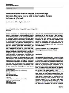
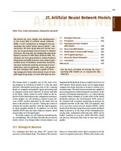
For neural networks, a partition is a group of neurons and G determines the number of neurons in the group. Landman and Russo define T as the number of connections (or pins) the partition forms with the rest of the network. The two parameters T and r are the Rent parameters with T defining the mean number of pins of a neuron and r determining the scaling of pin count with partition size. r is called the Rent exponent and is used as a measure of connection complexity (for other applications, see [1]): For low r (→ 0), pin count only slightly increases when partitions of the network are merged, meaning that most of the connections between them are internal to the combined partition. In other words, local connections dominate over global ones. In contrast, for high r (→ 1), merging partitions will produce only few internal connections. It is clear that the partitioning strategy also has an influence on the Rent exponent r. From the numerous possibilities (see [1]), we chose the method of Hagen et al. [14], because it promises the lowest possible r. In short, this method uses a spectra-based ratio cut algorithm to hierarchically divide a network into disjunct partitions with minimized connectivity between them. Then, a sequence of partitionings, i.e. complete divisions of the network into disjunct partitions, is extracted and average values G, T calculated for each; then, a straight-line fit of these values in the double-logarithmic domain gives the Rent parameters. In addition, we iteratively remove T -values deviating more than 5% from the fit. Figure 1A shows the restrictions on connectivity by a physical substrate: The substrate determines the maximum mean pins per element T sub by its relative
596
ESANN'2009 proceedings, European Symposium on Artificial Neural Networks - Advances in Computational Intelligence and Learning. Bruges (Belgium), 22-24 April 2009, d-side publi., ISBN 2-930307-09-9.
~rsub
B
log(Tout)
log(Tsub) log(T)
~r Region I
log(1)
pins per partition, T
pins per partition, T
A r = 0.86 T = 40
103
102
r = 0.86 T = 40
r =1 r =0.67
r =1 r =0.67
Region II
log(N) neurons per partition, G
101
100
101 102 neurons per partition, G
100
101 102 neurons per partition, G
Fig. 1: A: Qualitative scaling of pin count T with partition size G [2]. Gray area: allowed region of a substrate with maximum Rent parameters T sub and rsub . B: Partitions (points) and extracted partitioning sequences (lines) for twolevel networks with random (left) and neighbour (right) connectivity. Thin line: Extracted Rent power law. connection density, as well as the Rent exponent rsub by its dimension. For two dimensions, the exponent is restricted to r ≤ rsub = 12 ; otherwise, the fraction of connectivity on the whole system as well as the length of the connections must grow with network size [14], resulting in poor scaling. This is because pin count scales with system side length x, i.e. T ∼ x, but partition size scales with area, 1 i.e. G ∼ x2 , resulting in T ∼ G 2 . A similar argument leads to rsub = 23 for three-dimensional substrates [14]. The highest possible Rent exponent r = 1 is found in uniform random graphs and randomly partitioned networks [1]. Landman and Russo found the power law only for partitions up to a certain size, which they called Region I. For bigger partitions, a more complicated relationship is visible in their data, called Region II. As illustrated in Figure 1A, a reason for this effect may be the adaption of the internal connectivity to the often limited number of system inputs and outputs, Tout . The two-region solution also points to an obvious prerequisite of the power-law relationship that is often neglected: The connectivity at different system levels must be similar to make the relation work over a broad range of partition sizes (Region I). Otherwise, the solution has to be split up into more regions. We show this on a two-level model, for which the Rent exponents are known. On the lower level, groups of 5 neurons were fully connected (r = 1). On the higher level, groups were arranged on a 10 × 10 grid. 4 bi-directional inter-group connections were formed per group, either with nearest neighbours (r = 0.5) or with randomly chosen groups (r = 1). Figure 1B confirms our prediction that a single power law may not cover the whole connectivity.
4
Analysis results
We will now extract the relationship of pin count and partition size for the networks mentioned in section 2. For stochastic network models, we generated
597
ESANN'2009 proceedings, European Symposium on Artificial Neural Networks - Advances in Computational Intelligence and Learning. Bruges (Belgium), 22-24 April 2009, d-side publi., ISBN 2-930307-09-9.
A
B
105
104
d = 0.30 r = 0.90 T = 33
N = 1000 S = 135736 d = 13.6%
104
r = 0.976 T = 258
Kremkow et al. N = 1000 S = 70107 d = 7.0%
103
100
103
d = 0.15 r = 0.89 T = 40 local (d = 0) r = 0.83 T = 27
102 r =1
r = 0.974 T = 134
r =1 102
pins per partition, T
pins per partition, T
Häusler et al.
101 102 neurons per partition, G
101
103
100
N = 1000 S = 16702-25035 d = 1.7-2.5%
101 102 neurons per partition, G
C
103
D 103 r = 0.827 T = 14.3 pins per partition, T
pins per partition, T
104
103 r = 0.916 T = 28 102
101 100
r =1 101 102 neurons per partition, G
N = 1434 S = 43290 d = 2.1%
102
101
100
100
103
r =1 N = 277 S = 2105 d = 2.7% 101 neurons per partition, G
102
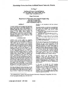
Fig. 2: Log-log plot of pin count over neuron count per partition for different networks; inlays denote basic network properties (N : neuron count, S: connection count, d: connection density, d = S/N 2 ); A: stochastic network models, B: displaced network model with different displacement distances d, C: HMAX network model, D: brain network of C. elegans. Points and lines as in Figure 1; single partitions omitted in A and B for clarity. instances with 1000 neurons and 100 inputs of the models by H¨ ausler and Maass [10] and Kremkow [11], using connection probabilities from the manuscripts. The resulting partitioning sequence is shown in Figure 2A. The Rent exponent is close to 1 in a wide range for both models due to the uniform random connectivity inside regions. Thus, linear (r = 1) scaling breaks down only at biggest partitions. The sharp decrease towards the biggest partition seen in the plot is caused by the low number of inputs and outputs to the network, which, however, has no influence on the partitioning at smaller partition sizes. To resemble the small-world model of Herzog et al. with displaced connections [12], we placed 1000 neurons on unit area [0, 1] × [0, 1], each having a branching point at distance d in random direction. A neuron connected to all neurons that were within distance 0.06 to its branching point. Figure 2B shows results for different branching point distances d. For pure local connectivity (d = 0), linear scaling breaks down at a partition size around 10 neurons, which roughly compares to the 11.3 neurons expected to lie inside the connection area. With increasing distance d, this break-down moves towards bigger partitions, making connectivity more random-like.
598
ESANN'2009 proceedings, European Symposium on Artificial Neural Networks - Advances in Computational Intelligence and Learning. Bruges (Belgium), 22-24 April 2009, d-side publi., ISBN 2-930307-09-9.
For analysing the routing complexity of hierarchical models, we generated a downscaled approximation of the HMAX model by Riesenhuber and Poggio [13]. Each layer was formed by a rectangular grid of neurons, which were connected according to a Gaussian probability function of increasing width at higher layers. As Figure 2C shows, the model has a high Rent exponent over a broad range. This may be caused by the randomness of connections and the high inter-layer connectivity. Only at the topmost partitionings, pin count per partition does not increase further with partition size, reflecting the structure in the network. Figure 2D shows partitioning results for the brain network of C. elegans [5]. It has a scaling with Rent exponent significantly lower than 1, but still high connection complexity. However, the increase lowers at a partition size of approximately 30 neurons. Common to all analysed models is a relatively high Rent exponent. Only at big partition sizes, the increase in connections per partition slows down, especially in the displaced connection model. Main reason for the high routing complexity is the random, unstructured connectivity at single connection level. While this connectivity reduces the complexity of the model description and is a reasonable assumption when fine-grained connectivity data is not feasible [11], it results in r → 1. This may not be a problem for present sizes of models (up to 10000 neurons), but could become critical if the models are scaled up by a few orders of magnitude. Interestingly, the network of C. elegans also has a relatively high Rent exponent. One reason for this may be that this brain network is very small compared to e.g. mammalian brains, making connectivity a weaker constraint than functional and other constraints.
5
Conclusion
In this paper, we used Rent’s Rule to analyse the routing complexity of neural network models. We found Rent exponents near to 1 (≥ 0.9) for most of the analysed models, which corresponds to a high routing complexity. Especially, such Rent exponents are much higher than would result from networks with constant connection density in a two- (r = 0.5) or three- (r = 0.67) dimensional substrate. Thus, most models scale poorly in such an environment. Some models showed a lower routing complexity at higher connection levels, which reflects the structure in the connectivity at system level. Our results pose several questions for future modeling: Can present spiking neural network models be scaled up without violating the connectivity constraints imposed by the brain as a three-dimensional substrate? Are there several fundamentally different connectivity levels in the brain or does the brain employ self-similarity at different network levels? Does biology decrease neuron density in bigger-size mammalian brains to allow for higher connection complexity than could be integrated in three dimensions (see Fig. 1)? Answering these questions will help in understanding the structure and the design constraints of biological neural networks as well as support their large-scale distributed simulation and implementation in neuromorphic hardware.
599
ESANN'2009 proceedings, European Symposium on Artificial Neural Networks - Advances in Computational Intelligence and Learning. Bruges (Belgium), 22-24 April 2009, d-side publi., ISBN 2-930307-09-9.
References [1] P. Christie and D. Stroobandt. The interpretation and application of Rent’s rule. IEEE transactions on VLSI systems, 8(6):639–648, 2000. [2] B.S. Landman and R.L. Russo. On a pin versus block relationship for partitions of logic graphs. IEEE transactions on computers, 20(12):1469– 1479, 1971. [3] M.E.J. Newman. The structure and function of complex networks. SIAM Review, 45:167–256, 2003. [4] Q. Wen and D.B. Chklovskii. Segregation of the brain into gray and white matter: A design minimizing conduction delays. PLOS Computational Biology, 1(7):617–630, 2005. [5] M. Kaiser and C.C. Hilgetag. Nonoptimal component placement, but short processing paths, due to long-distance projections in neural systems. PLOS Computational Biology, 2(7):805–815, 2006. [6] V. Braitenberg. Brain size and number of neurons: an exercise in synthetic neuroanatomy. Journal of Computational Neuroscience, 10:71–77, 2001. [7] V. Beiu and W. Ibrahim. Does the brain really outperform Rents rule? In ISCAS, pages 640–643, 2008. [8] J. Bailey and D. Hammerstrom. Why VLSI implementations of associative VLCNs require connection multiplexing. In ICNN, 2:173–180, 1988. [9] V. Beiu. 2D neural hardware versus 3D biological ones. In International symposium on neural computation, vienna, austria, 1998. [10] S. H¨ ausler and W. Maass. A statistical analysis of information-processing properties of lamina-specific cortical microcircuit models. Cerebral Cortex, 17(1):149–162, 2007. [11] J. Kremkow, A. Kumar, S. Rotter, and A. Aertsen. Emergence of population synchrony in a layered network of the cat visual cortex. Neurocomputing, 70:2069–2073, 2007. [12] A. Herzog, K. Kube, B. Michaelis, A.D. de Lima, and T. Voigt. Displaced strategies optimize connectivity in neocortical networks. Neurocomputing, 70:1121–1129, 2007. [13] M. Riesenhuber and T. Poggio. Hierarchical models of object recognition in cortex. Nature Neuroscience, 2(11):1019–1025, 1999. [14] L. Hagen, A.B. Kahng, J.K. Fadi, and C. Ramachandran. On the intrinsic Rent parameter and spectra-based partitioning methodologies. IEEE transactions on CAD of integrated circuits and systems, 13:27–37, 1994.
600