Then we'll give a formal definition of a cartesian vector — that is, a vector whose
... Here is shown a vector V together with an original cartesian coordinate ...
CHAPTER
1
On Vectors and Tensors, Expressed in Cartesian Coordinates
It’s not enough, to characterize a vector as “something that has magnitude and direction.” First, we’ll look at something with magnitude and direction, that is not a vector. Second, we’ll look at a similar example of something that is a vector, and we’ll explore some of its properties. Then we’ll give a formal definition of a cartesian vector — that is, a vector whose components we choose to analyse in cartesian coordinates. The definition can easily be generalized to cartesian tensors. Finally on this subject, we’ll explore some basic properties of cartesian tensors, showing how they extend the properties of vectors. As examples, we’ll use the strain tensor, the stress tensor, and (briefly) the inertia tensor. Figure 1.1 shows the outcome of a couple of rotations, applied first in one sequence, then in the other sequence. We see that if we add the second rotation to the first rotation, the result is different from adding the first rotation to the second rotation. So, finite rotations do not commute. They each have magnitude (the angle through which the object is rotated), and direction (the axis of rotation). But First rotation + Second rotation �= Second rotation + First rotation. However, infinitesimal rotations, and angular velocity, truly are vectors. To make this point, we can use intuitive ideas about displacement (which is a vector). Later, we’ll come back to the formal definition of a vector. What is angular velocity? We define ω as rotation about an axis (defined by unit vector l, say) with angular rate d� dt , where � is the angle through which the line P Q (see Figure 1.2) moves with respect to some reference position (the position of P Q at the reference time). So ω=
d� l, dt
and � = finite angle = �(t). 1
working pages for Paul Richards’ class notes; do not copy or circulate without permission from PGR
2004/9/8 21:28
2
Chapter 1 / ON VECTORS AND TENSORS, EXPRESSED IN CARTESIAN COORDINATES
Start
First rotation
Start
Second rotation
"First rotation"
Second rotation
First rotation
o
= rotate 90 about a vertical axis o
"Second rotation" = rotate 90 about a horizontal axis into the page
1.1 A block is shown after various rotations. Applying the first rotation and then the second, gives a different result from applying the second rotation and then the first.
FIGURE
To prove that angular velocity ω is a vector, we begin by noting that the infinitesimal rotation in time dt is ω dt = ld�. During the time interval dt (think of this as δt, then allow δt → 0), the displacement of P has amplitude Q P times d�. This amplitude is r sin θd�, and the direction is perpendicular to r and l, i.e. displacement = (ω ω × r)dt. Displacements add vectorially. Consider two simultaneous angular velocities ω 1 and ω 2. Then the total displacement (of particle P in time dt) is (ω ω1 × r)dt + (ω ω2 × r)dt = (ω ω1 + ω 2) × rdt for all r. We can interpret the right-hand side as a statement that the total angular velocity is ω 1 + ω 2. If we reversed the order, then the angular velocity would be the same sum, ω 2 + ω 1, associated with the same displacement, so ω 2 + ω 1 = ω 1 + ω 2. So: sometimes entities with magnitude and direction obey the basic commutative rule that A2 + A1 = A1 + A2, and sometimes they do not. What then is a vector? It is an entity that in practice is studied quantitatively in terms
working pages for Paul Richards’ class notes; do not copy or circulate without permission from PGR
2004/9/8 21:28
ON VECTORS AND TENSORS, EXPRESSED IN CARTESIAN COORDINATES
P r θ Q
O
l A rigid object is rotating about an axis through the the fixed point O.
1.2 P is a point fixed in a rigid body that rotates with angular velocity ω about an axis through O. The point Q lies at the foot of the perpendicular from P onto the rotation axis. FIGURE
3
3'
2' V 2
O
1' 1
1.3 Here is shown a vector V together with an original cartesian coordinate system having axes O x1 x2 x3 (abbreviated to O1, O2, O3). Also shown is another cartesian coordinate system with the same origin, having axes O x1� x2� x3� . Each system is a set of mutually orthogonal axes. FIGURE
of its components. In cartesians a vector V is expressed in terms of its components by V = V1xˆ 1 + V2xˆ 2 + V3xˆ 3
(1.1)
where xˆ i is the unit vector in the direction of the i-axis. An alternative way of writing equation (1.1) is V = (V1, V2, V3), and sometimes just the symbol Vi . Then V1 = V · xˆ 1 and in general Vi = V · xˆ i . Thus, when writing just Vi , we often leave understood (a) the fact that we are considering all three components (i = 1, 2, or 3); and (b) the fact that these particular components are associated with a particular set of cartesian coordinates. What then is the significance of working with a different set of cartesian coordinate axes? We shall have a different set of components of a given vector, V. See Figure 1.3 for an illustration of two different cartesian coordinate systems. What then are the new components of V?
working pages for Paul Richards’ class notes; do not copy or circulate without permission from PGR
2004/9/8 21:28
3
4
Chapter 1 / ON VECTORS AND TENSORS, EXPRESSED IN CARTESIAN COORDINATES
We now have V = V1�xˆ �1 + V2�xˆ �2 + V3�xˆ �3 where xˆ �1 is a unit vector in the new x �j – direction. So the new components are V j� . Another way to write the last equation is V = (V1�, V2�, V3�), which is another expression of the same vector V, this time in terms of its components in the new coordinate system. Then (a third way to state the same idea), V j� = V · xˆ �j .
(1.2)
We can relate the new components to the old components, by substituting from (1.1) into (1.2), so that V j� = (V1xˆ 1 + V2xˆ 2 + V1xˆ 3) · xˆ �j =
3 �
li j Vi
i=1
where li j = xˆ i · xˆ �j . Since li j is the dot product ot two unit vectors, it is equal to the cosine of the angle between xˆ i and xˆ �j ; that is, the cosine of the angle between the original xi –axis and the new x �j –axis. The li j are often called direction cosines. In general, l ji �= li j : they are not symmetric, because l ji is the cosine of the angle between the x j -axis and the xi� -axis, and in general this angle is independent of the angle between xi - and x �j -axes. But we don’t have to be concerned about the order of the axes, in the sense that cos(−θ) = cos θ so that li j is also the cosine of the angle between the x �j –axis and the xi –axis. At last we are in a position to make an important definition. We say that V is a cartesian vector if its components V j� in a new cartesian system are obtained from its components Vi in the previously specified system by the rule V j� =
3 �
li j Vi .
(1.3)
i=1
This definition indicates that the vector V has meaning, independent of any cartesian coordinate system. When we express V in terms of its components, then they will be different in different coordinate systems; and those components transform according to the rule (1.3). This rule is the defining property of a cartesian vector. It is time now to introduce the Einstein summation convention — which is simple to state, but whose utility can be appreciated only with practice. According to this convention, we don’t bother to write the summation for equations such as (1.3) which have a pair of repeated indices. Thus, with this convention, (1.3) is written V j� = li j Vi
working pages for Paul Richards’ class notes; do not copy or circulate without permission from PGR
2004/9/8 21:28
(1.4)
ON VECTORS AND TENSORS, EXPRESSED IN CARTESIAN COORDINATES
�3 and the presence of the “ i=1 ” is flagged by the once-repeated subscript i. Even though we don’t bother to write it, we must not forget that this unstated summation is still required over such repeated subscripts. [Looking ahead, we shall find that the rule (1.4) can be generalized for entities called second-order cartesian tensors, symbolized by A, with cartesian coordinates that differ in the new and original systems. The defining property of such a tensor is that its components in different coordinate systems obey the relationship A�jl = Aik li j lkl .] As an example of the summation convention, we can write the scalar product of two vectors a and b as a · b = ai bi . The required summation over i in the above equation, is (according to the summation convention) signalled by the repeated subscript. Note that the repeated subscript could be any symbol. For example we could replace i by p, and write ai bi = a p b p . Because it doesn’t matter what symbol we use for the repeated subscript in the summation convention, i or p here is called a dummy subscript. Any symbol could be used (as long as it is repeated). The Einstein summation convention is widely used together with symbols δi j and εi jk defined as follows:
δi j = 0
for i �= j,
and
δi j = 1
for i = j;
(1.5)
and εi jk = 0
if any of i, j, k are equal, otherwise
ε123 = ε312 = ε231 = −ε213 = −ε321 = −ε132 = 1.
(1.6)
Note that εi jk is unchanged in value if we make an even permutation of subscripts (such as 123 → 312), and changes sign for an odd permutation (such as 123 → 213). The most important properties of the symbols in (1.5) and (1.6) are then δi j a j = ai ,
εi jk a j bk = (a × b)i ,
for any vectors a and b; and the symbols are linked by the property � � � δil δ jl δkl � � � εi jk εlmn = �� δim δ jm δkm �� �δ δ jn δkn � in
(1.7)
(1.8)
from which it follows that εi jk εilm = δ jl δkm − δ jm δkl .
working pages for Paul Richards’ class notes; do not copy or circulate without permission from PGR
2004/9/8 21:28
(1.9)
5
6
Chapter 1 / ON VECTORS AND TENSORS, EXPRESSED IN CARTESIAN COORDINATES
To prove (1.8), note that if any pair of (i, j, k) or any pair of (l, m, n) are equal, then the left-hand side and right-hand side are both zero. (A determinant with a pair of equal rows or a pair of equal columns is zero.) If (i, j, k) = (l, m, n) = (1, 2, 3), then the left-hand side and right-hand side are both 1 because ε123ε123 = 1 and � � �1 0 0� � � � 0 1 0 � = 1. (1.10) � � �0 0 1� Any other example of (1.8) where the left-hand side is not zero, will require that the subscripts (i, j, k) be an even or an odd permutation of (1, 2, 3), and similarly for the subscripts (k, l, m), giving a value (for the left-hand side) equal either to 1 or to −1. But the same type of permutation of (i, j, k) or (l, m, n) (whether even or odd) will also apply to columns or to rows of (1.10), giving either 1 (for a net even permutation) or −1 (for a net odd permutation), and again the left-hand side of (1.8) equals the right-hand side. Because of the first of the relations given in (1.7), δi j is sometimes called the substitution symbol or substitution tensor. In recognition of its originator it also called the Kronecker delta. εi jk is usually called the alternating tensor. (1.9) follows from (1.8), recognizing that we need to allow for the summation over i. Thus � � � δii δ ji δki � � � εi jk εilm = �� δil δ jl δkl �� � �δ im δ jm δkm = δii (δ jl δkm − δ jm δkl ) − δ ji (δil δkm − δim δkl ) + δki (δil δ jm − δim δ jl ), but here δii is not equal to 1 (which is what most people who are unfamiliar with the �3 summation convention might think at first). Rather, δii = i=1 δii = δ11 + δ22 + δ33 = 3. Using this result, and the “substitution” property of the Kronecker delta function (the first of the relations in (1.7)), we find εi jk εilm = 3(δ jl δkm − δ jm δkl ) − (δ jl δkm − δ jm δkl ) + (δkl δ jm − δkm δ jl ), which simplifies to (1.9) after combining equal terms. As we should expect, the subscript i does not appear in the right-hand side. 1.1
Tensors
Tensors generalize many of the concepts described above for vectors. In this Section we shall look at tensors of stress and strain, showing in each case how they relate a pair of vectors. We shall develop (i)
the physical ideas behind a particular tensor (for example, stress or strain);
(ii)
the notation (for example, for the cartesian components of a tensor);
(iii)
a way to think conceptually of a tensor, that avoids dependence on any particular choice of coordinate system; and
working pages for Paul Richards’ class notes; do not copy or circulate without permission from PGR
2004/9/8 21:28
1.1
n
S x
Tensors
δ F = T δS
δS
S is an internal surface, inside a medium within which stresses are acting. δ S is a part of the surface S. x is the point at the center of δ S .
1.4 The definition of traction T acting at a point across the internal surface S with normal n (a unit vector). The choice of sign is such that traction is a pulling force. Pushing is in the opposite direction, so for a fluid medium, the pressure would be −n · T.
FIGURE
(iv)
the formal definition of a tensor (analogous to the definition of a vector based on (1.3) or (1.4)).
To analyze the internal forces acting mutually between adjacent particles within a continuum, we use the concepts of traction and stress tensor. Traction is a vector, being the force acting per unit area across an internal surface within the continuum, and quantifies the contact force (per unit area) with which particles on one side of the surface act upon particles on the other side. For a given point of the internal surface, traction is defined (see Fig. 1.4) by considering the infinitesimal force δF acting across an infinitesimal area δS of the surface, and taking the limit of δF/δS as δS → 0. With a unit normal n to the surface S, the convention is adopted that δF has the direction of force due to material on the side to which n points and acting upon material on the side from which n is pointing; the resulting traction is denoted as T(n). If δF acts in the direction shown in Fig. 1.4, traction is a pulling force, opposite to a pushing force such as pressure. Thus, in a fluid, the (scalar) pressure is −n · T(n). For a solid, shearing forces can act across internal surfaces, and so T need not be parallel to n. Furthermore, the magnitude and direction of traction depend on the orientation of the surface element δS across which contact forces are taken (whereas pressure at a point in a fluid is the same in all directions). To appreciate this orientation-dependence of traction at a point, consider a point P, as shown in Figure 1.5, on the exterior surface of a house. For an element of area on the surface of the wall at P, the traction T(n1) is zero (neglecting atmospheric pressure and winds); but for a horizontal element of area within the wall at P, the traction T(n2) may be large (and negative). Because T can vary from place to place, as well as with orientation of the underlying element of area needed to define traction, T is separately a function of x and n. So we write T = T(x, n). At a given position x, the stress tensor is a device that tells us how T depends upon n. But before we investigate this dependence, we first see what happens if n changes sign.
working pages for Paul Richards’ class notes; do not copy or circulate without permission from PGR
2004/9/8 21:28
7
8
Chapter 1 / ON VECTORS AND TENSORS, EXPRESSED IN CARTESIAN COORDINATES
n2 P n1
1.5 T(n1) �= T(n2). The traction vector in general is different for different orientations of the area across with the traction is acting. FIGURE
n T(n)
T( – n) –n
1.6 A disk with parallel faces. The normals to opposite faces have the same direction but opposite sign.
FIGURE
By considering a small disk-shaped volume (Figure 1.6) whose opposite faces have opposite normals n and −n, we must have a balance of forces T(−n) = −T(n)
(1.11)
otherwise the disk would have infinite acceleration, in the limit as its volume shrinks down to zero. (There is negligible effect from the edges as they are so much smaller than the flat faces.) In a similar fashion we can examine the balance of forces on a small tetrahedron that has three of its four faces within the planes of a cartesian coordinate system, as shown in Figure 1.7. The oblique (fourth) face of the tetrahedron has normal n (a unit vector), and by projecting area ABC onto each of the coordinate planes, we find the following relation between areas:
working pages for Paul Richards’ class notes; do not copy or circulate without permission from PGR
2004/9/8 21:28
1.1
Tensors
2 3
n
C
B T(n)
O
T(– xˆ 2 )
1
A
– xˆ 2
1.7 The small tetrahedron O ABC has three of its faces in the coordinate planes, with outward normals −ˆx j ( j = 1, 2, 3) (only one of which is shown here, j = 2), and the fourth face has normal n.
FIGURE
(O BC, OC A, O AB) = ABC (n 1, n 2, n 3).
(1.12)
There are four forces acting on the tetrahedron, one for each face. Thus, face O BC has the outward normal given by the unit vector −ˆx1 = (−1, 0, 0). This face is pulled by the traction T(−ˆx1), and hence by the force T(−ˆx1) times area O BC (remember, traction is force per unit area). The balance of forces then requires that T(n) ABC + T(−ˆx1) O BC + T(−ˆx2) OC A + T(−ˆx3) O AB = 0.
(1.13)
(If the right-hand side were not zero, we would get infinite acceleration in the limit as the tetrahedron shrinks down to the point O.) Using the two equations (1.11)–(1.13), it follows that T(n) = T(ˆx1)n 1 + T(ˆx2)n 2 + T(ˆx3)n 3 = T(ˆx j )n j
(using the summation convention).
(1.14)
If we now define τkl = Tl (ˆxk ),
(1.15)
Ti (n) = τ ji n j .
(1.16)
Ti = τi j n i .
(1.17)
then
If we can show that τ ji = τi j , then
working pages for Paul Richards’ class notes; do not copy or circulate without permission from PGR
2004/9/8 21:28
9
10
Chapter 1 / ON VECTORS AND TENSORS, EXPRESSED IN CARTESIAN COORDINATES
This equation gives a simple rule by which the components of the traction vector, Ti , are given as a linear combination of the components of the normal vector n j . The nine symbols τi j are the cartesian components of a tensor, namely, the stress tensor. First, we’ll show that indeed τ ji = τi j . Second, we’ll show that the symbols τi j specify a surface which is independent of our particular choice of coordinate axes.
1.1.1
SYMMETRY OF THE STRESS TENSOR
To see why the τi j are symmetric, we can look in some detail at a particular example, namely τ21 and τ12. They quantify components of the tractions T (force per unit area) acting on the faces of a small cube with sides of length δx1, δx2, δx3 as shown in Figure 1.8. The force acting on the top face of the cube is traction × area, which is T(ˆx2) δx1 δx2. ˆ 2) δx1 δx2. From these two faces, what is the And on the opposite face the force is T(−x strength of the resulting couple that tends to make the cube rotate about the x3 axis? The x2 and x3 components of T have no relevance here (they are associated with the tendency to rotate about different axes) — only the x1 component of T, which is τ21. Figure 1.8b shown the resulting couple, and it is τ21 δx1 δx2 δx3 in the negative x3 direction. When we look at the tractions acting on the right and left faces, as shown in Figure 1.8c, the couple that results (see Fig. 1.8d) is τ12 δx1 δx2 δx3 in the positive x3 direction. No other couple is acting in the x3 direction, so the two couples we have obtained must be equal and opposite, otherwise the cube would spin up with increasing angular velocity. It follows that τ21 = τ12. By similar arguments requiring no net couple about the x1 or x2 directions, we find τ32 = τ23 and τ31 = τ13. So in general, τ ji = τi j and we have proven the symmetry required to obtain (1.17) from (1.16).
1.1.2
NORMAL STRESS AND SHEAR STRESS
Figure 1.9 shows two components of a traction vector T, one in the normal direction, and the other in the direction parallel to the surface across which T acts. The normal stress, σn , is given by σn = component of traction in the normal direction =T·n
(1.18)
= Tjn j = τi j n i n j .
Note that normal stress, as defined here, is a scalar. But it is associated with a particular direction, and the vector σn n is often used for the normal stress (as shown in Figure 1.9). The shear stress is the component of T in the plane of the surface across which traction is acting, so it may be evaluated by subtracting the normal stress σn n from T itself: shear stress = T − (T · n) n.
working pages for Paul Richards’ class notes; do not copy or circulate without permission from PGR
2004/9/8 21:28
(1.19)
1.1
Tensors
2
xˆ 2 T(xˆ 2 )
(a)
(b) area = δx1 δx 3
δx1
3
T(– xˆ 2)
δx 2 δx 3
τ 21 distance = δx 2
1 τ 21
– xˆ 2
2
(d)
(c)
τ 12
T(xˆ 1 ) – xˆ 1
δx 2 δx1
δx 3
distance = δx 1
xˆ 1
area = δx2 δx 3 1
T(– xˆ 1) τ
12
3
1.8 A small cube is shown, with an analysis of the couple tending to make the cube spin about the O x3 axis. Thus, in (a) is shown the tractions acting on the top and bottom faces. In (b) is shown the couple associated with these tractions which will tend to make the cube rotate about the axis into the plane of the page — the couple consists of a pair of forces τ21δx1 δx3 separated by a distance δx2. In (c) is shown the tractions acting on the right and left faces, and in (d) the associated couple tending to make the cube rotate about an axis out of the plane of the page. FIGURE
working pages for Paul Richards’ class notes; do not copy or circulate without permission from PGR
2004/9/8 21:28
11
12
Chapter 1 / ON VECTORS AND TENSORS, EXPRESSED IN CARTESIAN COORDINATES
T(n) normal stress = (T(n).n) n
shear stress = T – (T(n).n) n
1.9 The traction T is shown resolved into its normal and shear components.
FIGURE
P n normal to Σ at P
O Σ
1.10 � is a “quadric surface” centered on the coordinate origin O. P is the point on � at the place where a line drawn from the origin in the direction of n (a unit vector) meets the quadric surface. The normal to � at P is shown, and in general it will be in a direction different from the direction of n. FIGURE
It is unfortunate that the word “stress” is used for scalar quantities as in (1.18), for vector quantities as in (1.19), and for tensor quantities as in (1.15). In a fluid with no viscosity, the scalar normal stress is equal to pressure (but with opposite sign, in our convention where traction is positive if it is pulling). And in such a fluid, the shear stresses are all zero. 1.1.3
A QUADRIC SURFACE ASSOCIATED WITH THE STRESS TENSOR
The surface � given by the equation τi j xi x j = constant
(1.20)
has properties that are independent of the coordinate system used to define components xi and τi j . � is a three-dimensional surface, either a spheroid or a hyperboloid (which may have one or two separate surfaces). Because (1.20) has no linear terms (terms in xi only), � is a surface which is symmetric about the origin O, as shown in Figure 1.10. (If x is a point on the surface �, then so is the point −x.) If P is at position x, then
working pages for Paul Richards’ class notes; do not copy or circulate without permission from PGR
2004/9/8 21:28
1.1
Tensors
1.1 On finding the direction of a normal to a surface
BOX
If � is the surface composed of points x which satisfy the equation F(x) = c for some constant c, then consider a point x + δx which also lies on �. Then F(x + δx) = c, so F(x + δx) − F(x) = 0. But F(x + δx) = F(x) + δxi
∂F ∂ xi
(Taylor series expansion)
= F(x) + δx · ∇ F. Therefore, δx · ∇ F = 0 for all directions δx such that x and x + δx lie in the surface �. Since δx is tangent to � at the point x, and δx · ∇ F = 0 for all such tangents, this last equantion shows that ∇ F has the defining property of the normal to � at x (it is perpendicular to all the tangents at x). We conclude that the normal to the surface F(x) = c is parallel to ∇ F.
vector OP = x = OP n
(1.21)
and the length OP is related to the normal stress. This follows, because constant = τi j xi x j = τi j OP n i OP n j = OP2 τi j n i n j = OP2 σn
from (1.18).
Hence, σn ∝
1 . OP2
(1.22)
This is a geometrical property of �, which depends only the shape of the quadric surface, not its absolute size. Another such geometrical property is associated with the normal to � at P. We can use Box 1.1 to see that this normal is in the direction whose i-th component is
working pages for Paul Richards’ class notes; do not copy or circulate without permission from PGR
2004/9/8 21:28
13
14
Chapter 1 / ON VECTORS AND TENSORS, EXPRESSED IN CARTESIAN COORDINATES
∂ ∂ xk ∂ xl (τkl xk xl ) = τkl xl + τkl xk ∂ xi ∂ xi ∂ xi = τkl δik xl + τkl xk δil = τil xl + τki xk = 2τi j x j
(the partial derivatives are Kronecker delta functions)
(using the substitution property (1.7))
(using symmetry of the stress tensor, and changing dummy subscripts)
= 2OP τi j n j = 2OP Ti
(chain rule)
(from (1.21)) (from (1.17)).
It follows that the normal to � at P is parallel to the traction vector, T.
(1.23)
The results (1.22) and (1.23) are the two key geometrical features of the quadric surface representing the underlying tensor τ , and they are independent of any coordinate system. Going back to Figures 1.4 and 1.9, the quadric surface shown in Figure 1.10 is a geometrical device for obtaining the direction of the traction vector, and the way in which normal stress varies as the unit normal n varies (specifying the orientation of an area element across which the traction acts). We can for example see geometrically that there are three special directions n, for which the traction T(x) is parallel to n and hence (for these n directions) the shear stress vanishes. To obtain the same result algebraically, we note that these special values of n are such that Ti ∝ n i and so, using (1.17), τi j n j = λn i .
(1.24)
As discussed in Box 1.2, this last equation has solutions (for n), but only if λ takes on one of three special values (eigenvalues); and the three resulting values of n (one for each λ value) are mutually orthogonal. 1.1.4
FORMAL DEFINITION OF A SECOND ORDER CARTESIAN TENSOR
If two cartesian coordinate systems O x1 x2 x3 and O x1� x2� x3� are related to each other as shown in Figure 1.3, with direction cosines defined by li j = xˆ i · xˆ j , then the entity A is a second order cartesian tensor if its components Aik in the O x1 x2 x3 system and A�jl in the O x1� x2� x3� system are related to each other by A�jl = Aik li j lkl .
(1.25)
It is left as an exercise (in Problem 1.1) to obtain the reverse transformation, and to show that the associated quadric surface Ai j xi x j = c is given also by Ai� j xi� x �j = c. The tensor A is isotropic if its components are the same in the original and the transformed coordinate systems. It follows geometrically that the quadric surface of such a tensor is simply a sphere, and that Ai j = Ai� j = constant × δi j . The stress tensor in an inviscid fluid is isotropic (Problem 1.4 asks you to prove this).
working pages for Paul Richards’ class notes; do not copy or circulate without permission from PGR
2004/9/8 21:28
1.1
Tensors
1.2 On solutions of
BOX
A · x = λx where A is a symmetric real matrix Here we briefly review the main properties of the set of linear equations Ai j x j = λxi
(where A ji = Ai j ; i = 1, . . . , n; and j = 1, . . . , n).
(1)
These are n equations in n unknowns. In the present chapter, usually n = 3. Equation (1) is fundamentally different from the standard linear problem A · x = b, or Ai j xi = bi ,
(2)
which has a straightforward solution provided det A �= 0, for then the inverse matrix exists and x = A−1 · b. Note that for equation (1) there is no restriction on the absolute size of x: if x is a solution of (1), then so is cx for any constant c. But if x is a solution of (2), then in general cx will not be a solution. Equation (1) has the trivial solution x = 0, but we are interested in non-trivial solutions, for which at least one component of x is non-zero. It follows that equation (1) represents a set of n scalar relations between n − 1 variables, for example x j /x1 ( j = 2, . . . , n). If x1 = 0 then we can instead divide (1) by some other component of x. We can use the Kronecker delta function to write (1) as (Ai j − λδi j )x j = 0,
(A − λI) · x = 0,
or as
(1, again)
where I is the identity matrix, Ii j = δi j , with 1 at every entry on the diagonal and 0 everywhere else. If det (A − λI) �= 0, then the inverse (A − λI)−1 exists and the only solution of (1) is x = (A − λI)−1 · 0, giving x = 0. It follows that the only way we can obtain non-trivial solutions of (1), is to require that det (A − λI) = 0.
(3)
Equation (3) is an n-th order polynomial in λ, and in general it has n solutions, λ(α) (α = 1, . . . , n), called eigenvalues of the matrix A. For each eigenvalue, we have an associated eigenvector x(α) satisfying A · x(α) = λ(α)x(α)
(not summed over α).
(4)
These eigenvectors (there are n of them, since α = 1, . . . , n) are the vector solutions of (1), so they have the special property that A · x(α) is in the same direction as the vector x(α) itself. Equation (1) imposes no contraint on the absolute size of solutions such as x(α), and we are free to normalize these solutions if we wish. A common choice is to make x(α) · x(α) = 1. The final important property of the eigenvectors, is that any two eigenvectors corresponding to two different eigenvalues must be orthogonal. To prove this, we consider two eigenvalues λ(α) and λ(β) with corresponding eigenvectors x(α) and x(β), and λ(α) �= λ(β). Then (α) (α) Ai j x (α) j = λ xi
and
working pages for Paul Richards’ class notes; do not copy or circulate without permission from PGR
(β)
Ai j x j
2004/9/8 21:28
(β)
= λ(β)xi .
(5)
15
16
Chapter 1 / ON VECTORS AND TENSORS, EXPRESSED IN CARTESIAN COORDINATES
BOX
1.2 (continued) (β)
We can multiply both sides of the first of equations (5) by xi and sum over i, and multiply both sides of the second of equations (5) by xi(α) and sum over i, giving (β)
Ai j x (α) j xi
(β)
= λ(α)x(α) · x(β)
(6a)
(β)
= λ(β)x(α) · x(β).
(6b)
= λ(α) xi(α) xi
and (β)
Ai j x j xi(α) = λ(β) xi(α) xi
Note here that we are using the Einstein summation convention in the usual way for repeated subscripts, but we are not using it for repeated superscripts α and β. [The summation convention does not work naturally with such superscripts, because one side of equations such as (4) or (6a) has repeated superscripts, and the other side has the superscript in just one place.] (β) (β) Because A is a symmetric matrix, Ai j x j xi(α) = A ji x j xi(α). But we can use any symbol for repeated subscripts, and in particular we can exchange the symbols i and j in this last (β) (β) (β) (β) expression, so that Ai j x j xi(α) = A ji x j xi(α) = Ai j x j xi(α) = Ai j xi(α) x j . Hence, the lefthand side of (6a) equals the left-hand side of (6b). Subtracting (6b) from (6a), we see that (λ(α) − λ(β)) x(α) · x(β) = 0. But the first of these factors is not zero, since we took the eigenvalues to be different (λ(α) �= λ(β)). It follows that the second factor must be zero, x(α) · x(β) = 0, and hence that the eigenvectors corresponding to different eigenvalues are orthogonal. The best way to become familiar with the eigenvalue/eigenvector properties described above, is to work through the details of a few examples (such as Problem 1.2).
The above formal definition of a tensor is rarely useful directly, as a way to demonstrate that an entity (suspected of being a tensor) is in fact a tensor. For this purpose, we usually rely instead upon the so-called quotient rule, which states that if the relationship Tik Ak = Bi is true is all coordinate systems, where Ak and Bi are the components of vectors A and B, then the Tik are components of a second order cartesian tensor provided the components of A can all be varied separately. The statement that “the relationship Tik Ak = Bi is true is all � A� = B � as well as T A = B . coordinate systems” means that T jk ik k i l j To show that the quotient rule means the formal definition is satisfied, note that � T jk Al� = B �j
= Bi li j
since B is a vector
= Tik Ak li j
using Tik Ak = Bi
= Tik Al� lkl li j
from the reverse transform Ak = Al� lkl — see Problem 1.1.
Hence
working pages for Paul Richards’ class notes; do not copy or circulate without permission from PGR
2004/9/8 21:28
1.2
The strain tensor
Q
u(x + δx)
Q0 δx
P0 u(x)
P
x
O
1.11 A line element δx is shown with ends at P0 and Q 0, and also after the neighborhood of P0 has undergone deformation. The new position of the line element is from P to Q. P0 is at x, Q 0 is at x + δx, P is at x + u and Q is at x + δx + u(x + δx). FIGURE
(T jl� − Tik li j lkl )Al� = 0.
(1.26)
This is a set of three scalar equations ( j = 1, 2, or 3). But since they are also true as the components Al� are varied independently, it follow that the coefficients of the Al� (l = 1, 2, or 3) must all vanish. So T jl� = Tik li j lkl , and T satisfies the formal definition of a tensor (compare with (1.25)). The entity we have been calling the stress tensor, τ , satisfies the quotient rule (see equation (1.17), in which the components of τ relate the traction vector and n). It is for this reason that indeed we are justified in referring to τ as a second order cartesian tensor. 1.2
The strain tensor
Two different methods are widely used to describe the motions and the mechanics of motion in a continuum. These are the Lagrangian description, which emphasizes the study of a particular particle that is specified by its original position at some reference time, and the Eulerian description, which emphasizes the study of whatever particle happens to occupy a particular spatial location. Note that a seismogram is the record of motion of a particular part of the Earth (namely, the particles to which the seismometer was attached during installation), so it is directly a record of Lagrangian motion. A pressure gauge attached to the sea floor also provides a Lagrangian record, as does a neutrally buoyant gauge that is free to move in the water. But a gauge that is fixed to the sea floor and measuring properties (such as velocity, temperature, opacity) of the water flowing by, provides an Eulerian record. We use the term displacement, regarded as a function of space and time, and written as u = u(x, t), to denote the vector distance of a particle at time t from the position x that it occupies at some reference time t0, often taken as t = 0. Since x does not change with time, it follows that the particle velocity is ∂u/∂t and that the particle acceleration is ∂ 2u/∂t 2. To analyze the distortion of a medium, whether it be solid or fluid, elastic or inelastic,
working pages for Paul Richards’ class notes; do not copy or circulate without permission from PGR
2004/9/8 21:28
17
18
Chapter 1 / ON VECTORS AND TENSORS, EXPRESSED IN CARTESIAN COORDINATES
we use the strain tensor. If a particle initially at position x is moved to position x + u, then the relation u = u(x) is used to describe the displacement field. To examine the distortion of the part of the medium that was initially in the vicinity of x, we need to know the new position of the particle that was initially at x + δx, where δx is a small line-element. This new position (see Figure 1.11) is x + δx + u(x + δx). Any distortion is liable to change the relative position of the ends of the line-element δx. If this change is δu, then δx + δu is the new vector line-element, and by writing down the difference between its end points we obtain δx + δu = x + δx + u(x + δx) − (x + u(x)). Since |δx| is arbitrarily small, we can expand u(x + δx) as u + (δx · ∇)u plus negligible terms of order |δx|2. It follows that δu is related to gradients of u and to the original lineelement δx via δu = (δx · ∇)u,
δu i =
or
∂u i δx j . ∂x j
(1.27)
However, we do not need all of the nine independent components of ∂∂ux ij to specify true distortion in the vicinity of x, since part of the motion is due merely to an infinitesimal rigid-body rotation of the neighborhood of x. We shall write δu i =
∂u i δx j = ∂x j
� 1 2
∂u j ∂u i + ∂x j ∂ xi
�
� δx j +
1 2
∂u j ∂u i − ∂x j ∂ xi
� δx j
and use the result given in Problem 1.8 to interpret the last term of the above equation. Introducing the notation u i, j for ∂∂ux ij , we then see that (1.27) can be rewritten as δu i = 12 (u i, j + u j,i )δx j + 12 (curl u × δx)i ,
(1.28)
and the rigid-body rotation is of amount �12 curl� u. The interpretation of the last term in (1.28) as a rigid-body rotation is valid if �u i, j � � 1. If displacement gradients were not “infinitesimal” in the sense of this inequality, then we would instead have to analyze the contribution to δu from a finite rotation—a much more difficult matter, since finite rotations do not commute and cannot be expressed as vectors. In terms of the infinitesimal strain tensor, defined to have components ei j ≡ 12 (u i, j + u j,i ),
(1.29)
the effect of true distortion on any line-element δx is to change the relative position of its end points by a displacement whose i-th component is ei j δx j . By the quotient rule discussed in Section 1.1.4, it follows that e is indeed a second order cartesian tensor. Rotation does not affect the length of the element, and the new length is
working pages for Paul Richards’ class notes; do not copy or circulate without permission from PGR
2004/9/8 21:28
1.2
√ δx · δx + 2δu · δx � = δxi δxi + 2ei j δxi δx j
|δx + δu| =
= |δx| (1 + ei j νi ν j )
The strain tensor
(neglecting δu · δu) (from (1.28), and using (curl u × δx) · δx = 0) � � (to first order, if � ei j � � 1),
where ν is the unit vector δx/ |δx|. It follows that the extensional strain of a line-element originally in the ν direction, which we define to be e(νν ) =
change in length PQ − P0 Q 0 , = original length P0 Q 0
is given by e(νν ) = ei j νi ν j .
(1.30)
Strain is a dimensionless quantity. The diurnal solid Earth tide leads to strains of about 10−7. Strains of about 10−11 due to seismic surface waves from distant small earthquakes can routinely be measured with modern instruments. 1.2.1
THE STRAIN QUADRIC
We can define the surface ei j xi x j = constant. If it is referred to the axes of symmetry as coordinate axes, this quadric surface becomes E 1 x12 + E 2 x22 + E 3 x32 = constant and the strain tensor components become E1 0 0 e = 0 E2 0 . 0 0 E3 The E i (i = 1, 2, or 3), called principal strains, are eigenvalues of the matrix e11 e12 313 e = e12 e22 323 e13
e23
333
(this matrix is different for different cartesian coordinate systems, but its eigenvalues are the same). Figure 1.12 shows an example of the strain quadric, in the case that the E i do not all have the same sign. In this case, � is a hyperboloid. The figure caption describes the two key geometrical properties of �, analogous to the results shown previously for the stress quadric (see (1.22) and (1.23)). The first property, e(νν ) ∝ OP−2, follows from taking x = OPνν and substituting for the components of x in ei j xi x j = constant. The second property, concerning the direction of the displacement due to distortion, follows from showing that the direction of the normal at P is parallel to ∇(ei j xi x j ), which has i-th component 2ei j x j = 2OPei j ν j . In terms of the line-element δx, this i-th component is proportional to ei j δx j , and indeed this is in the displacement direction due to the distortion (see comments following (1.29)). The physical interpretation of the axes of symmetry of �, is that these are the three special (mutually orthogonal) directions in which an original line-element is merely
working pages for Paul Richards’ class notes; do not copy or circulate without permission from PGR
2004/9/8 21:28
19
20
Chapter 1 / ON VECTORS AND TENSORS, EXPRESSED IN CARTESIAN COORDINATES
principal axis #2
principal axis #1
O
ν
P
Σ
1.12 A hyperboloid is shown here, as an example of a strain quadric �. The third principal axis is perpendicular to the first two (out of the page). For a line-element in the ν direction, extensional strain is inversely proportional to OP2. The displacement of the end of the line-element, due to distortion, is in the direction of the normal at P.
FIGURE
shortened or lengthened by the deformation. For these special directions, line-elements are not subject to any shearing motions. The only rotation, is that which applies to the whole neighborhood of the line-element as a rigid body rotation (distinct from deformation). 1.3
Some simple examples of stress and strain
Examples are (i)
Compacting sediments, which shrink in the vertical direction but stay the same in the horizontal direction. Think of them as being in a large tank (see Figure 1.13). If x1 and x2 are horizontal directions with x3 vertical, then the strain tensor has components 0 0 0 e = 0 0 0 . 0 0 e33 Compression at depth, from the weight of those above, leads to e33 < 0. But although the strain tensor has only one non-zero component, the stress tensor has non-zero values of τ11, τ22, τ33. If the sediments lack strength, then the stress will essentially be the same as if the material were composed of a fluid (lacking any ability to resist shearing forces). In this case, the stress at depth x3 is due solely to pressure generated by the overburden. There are no shearing forces, and x3 P 0 0 τ =− 0 P 0 where P = ρg dx3. 0 0 0 P
working pages for Paul Richards’ class notes; do not copy or circulate without permission from PGR
2004/9/8 21:28
1.3
Some simple examples of stress and strain
x3
1.13 Sediments, compressed vertically.
FIGURE
(ii)
A wire that is stretched in the x1−direction will shrink in the perpendicular directions x2 and x3. The strain tensor is
e11 e= 0 0
0 e22 0
0 0 , e33
with e11 > 0 and e22 = e33 < 0.
The stress tensor has only one non-zero component:
τ11 τ = 0 0 (iii)
0 0 0
0 0. 0
We use the term pure shear to describe the type of deformation shown in Figure 1.14, in which a small rectangle is subjected to the stress field
0 τ = τ12 0
τ12 0 0
0 0. 0
In this deformation, the point B has moved to the right from its original position, by ∂u 1 ∂u 2 an amount δx2, and the point A has moved up an amount δx1. In the case ∂ x2 ∂ x1 of pure shear, there is no rigid body rotation. So curl u = 0 which means here that ∂u 1 ∂u 2 = . The line element OB0 has been rotated over to the right (clockwise) ∂ x2 ∂ x1 ∂u 1 ∂u 1 by an angle given by δx2 ÷ δx2 = . The line element O A0 has been rotated ∂ x2 ∂ x2 ∂u 2 ∂u 2 ∂u 1 anticlockwise by the angle δx1 ÷ δx1 = = since there is no rigid body ∂ x1 ∂ x1 ∂ x2 rotation, and the strain tensor components are
0 e = e21 0
e12 0 0
0 0. 0
∂u 1 ∂u 2 = . ∂ x2 ∂ x1 The reduction in the original π/2 angle at O (Figure 1.14) is 2e12. The ratio between stress and this angle reduction,
Always, e ji = ei j . And for pure shear, e12 = e21 =
working pages for Paul Richards’ class notes; do not copy or circulate without permission from PGR
2004/9/8 21:28
21
22
Chapter 1 / ON VECTORS AND TENSORS, EXPRESSED IN CARTESIAN COORDINATES
x2
x2
original shape
deformed shape (pure shear) B
B0 δx2
A
O
δx1
A0
O
x1
x1
1.14 A small rectangular prism is sheared with no change in area. The shearing stresses τ12 and τ21(= τ12) are the same as those shown in Figure 1.8b and 1.8d. FIGURE
x2
x2
angle = e12
angle = 2 e12
δx2 angle = e12 O
δx1
O
x1
simple shear
x1 pure shear as shown above, plus a clockwise rotation of the whole block through an angle e12
=
1.15 A simple shear is shown on the left, with u 1 ∝ x2, so that an original rectangle in the O x1 x2-plane is now sheared with motion only in the x1-direction. This motion is equivalent to a pure shear followed by a clockwise rigid-body rotation. The angle reduction at the origin is 2e12 in both cases. Rigidity is the ratio between shear stress and the angle reduction. For a viscous material, the material continues to deform as long as the shear stress is applied, and viscosity is defined as the ratio between shear stress and the rate of angle reduction. FIGURE
µ=
τ12 , 2e12
(1.31)
is known as the rigidity. (iv)
Consider a deformation in which the displacement is u = (u 1, 0, 0) and u 1 depends on x only via the x2-component. An example is shown in Figure 1.15, and this situation is called a simple shear. It can be regarded as a pure � by � shear described 1 ∂u 1 1 ∂u 1 . e12 = e21 = , plus a rigid rotation of amount 12 curl u = 0, 0, − 2 ∂ x2 2 ∂ x2 The definition of rigidity is easier to understand with a simple shearing defor∂u 1 mation. It is the shearing stress τ21 divided by the displacement gradient (equal ∂ x2 to the angle reduction as shown in Figure 1.15).
working pages for Paul Richards’ class notes; do not copy or circulate without permission from PGR
2004/9/8 21:28
1.4
extension (strain)
Relations between stress and strain
strain hardening onset of yielding
Rubber
Steel
strain weakening
force (tension, stress)
1.16 For some solid materials, strain grows in proportion to stress at low stress, but the linearity is lost and strain either increases more slowly with increasing stress (for example, rubber), or increases more quickly (for example, steel). At high enough stress, the material breaks. This is a schematic diagram: some solids break at extensional strains as small as 10−3, and some forms of rubber maintain linearity even for strains of order 1. FIGURE
All of the above examples in this subsection are elastic examples. Stress and strain go to zero together, if τi j = ci jkl ekl , and there is no time-dependence. Real materials can be quite different, exhibiting viscous behavior, or strain hardening, or a tendency to yield at high values of applied stress (see Figure 1.16). We take up this subject next, with emphasis on solids. 1.4
Relations between stress and strain
A medium is said to be elastic if it possesses a natural state (in which strains and stresses are zero) to which it will revert when applied forces are removed. Under the influence of applied loads, stress and strain will change together, and the relation between them, called the constitutive relation, is an important characteristic of the medium. Over 300 years ago, Robert Hooke summarized the relationship today known as Hooke’s Law between the extension of a spring, and the force acting to cause the extension. He concluded experimentally that force ∝ extension. The constant of proportionality here is often called a modulus, M (say), and then force = M × extension. (Hooke’s Law appeared originally as an anagram, ceiiinosssttuv, of the Latin phrase ut tensio, sic vis — meaning “as the extension, so the force.” Some scientific personalities are very strange.) The modern generalization of Hooke’s law is that each component of the stress tensor is a linear combination of all components of the strain tensor, i.e., that there exist constants ci jkl such that τi j = ci j pq e pq .
(1.32)
A material that obeys the constitutive relation (1.32) is said to be linearly elastic. The
working pages for Paul Richards’ class notes; do not copy or circulate without permission from PGR
2004/9/8 21:28
23
24
Chapter 1 / ON VECTORS AND TENSORS, EXPRESSED IN CARTESIAN COORDINATES
quantities ci jkl are components of a fourth-order tensor, and have the symmetries c ji pq = ci j pq
(due to τ ji = τi j )
(1.33)
(due to eq p = e pq ).
(1.34)
and ci jq p = ci j pq
It is also true from a thermodynamic argument that c pqi j = ci j pq ,
(1.35)
for a material in which the energy of deformation (associated with tensors τ and e) does not depend on the time history of how the deformation was acquired. The ci jkl are independent of strain, which is why they are sometimes called “elastic constants,” although they are varying functions of position in the Earth. In general, the symmetries (1.33), (1.34), and (1.35) reduce the number of independent components in ci jkl from 81 to 21. There is considerable simplification in the case of an isotropic medium, since c must be isotropic. It can be shown that the most general isotropic fourth-order tensor, having the symmetries of c, has the form ci jkl = λδi j δkl + µ(δik δ jl + δil δ jk ).
(1.36)
This involves only two independent constants, λ and µ, known as the Lam´e moduli. Substituting from (1.36) into (1.32), we see that the stress–strain relation becomes τi j = λδi j ekk + 2µei j
(1.37)
in isotropic elastic media. If we consider only shearing stresses and shearing strains, using (1.37) with i �= j, then τi j = 2µei j and µ here is just the rigidity we introduced earlier, in (1.31). For many materials, the Lam´e moduli λ and µ (sometimes called Lam´e constants) are approximately equal. They can be used to generate a number of other constants that characterize the properties of material which are subjected to particular types of strain and stress, for example the stretched wire discussed as item (ii) of Section 1.3. For that example, (1.37) gives τ11 = λ(e11 + e22 + e33) + 2µe11 0 = λ(e11 + e22 + e33) + 2µe22
(1.38)
0 = λ(e11 + e22 + e33) + 2µe33. By comparing the second and third of these equations, we see that e22 = e33; and then from these same two equations it follows that λe11 + 2(λ + µ)e22 = 0. Poisson’s ratio is defined as ν=
working pages for Paul Richards’ class notes; do not copy or circulate without permission from PGR
shrinking strain stretching strain
2004/9/8 21:28
Problems
in this example of simple stretching, so ν=
−e22 λ 1 = ∼ e11 2(λ + µ) 4
(1.39)
if λ and µ are approximately equal (which is the case for many common materials). Another important class of materials is that for which shearing stresses lead to flow. Such materials are not elastic. We introduce the deviatoric stress as the difference between τi j and the average of the principal stresses, which is 13 τkk and which we can symbolize by −P. (In an inviscid or perfect fluid, P with this definition is simply the scalar pressure.) The viscosity of a material that can flow, such as syrup (with low viscosity) or the Earth’s mantle (with high viscosity, and significant flow occurring only over many millions of years), is the constant of proportionality between the deviatoric stress and twice the strain rate. Thus, the viscosity ν is given by τi j + Pδi j = 2ν e˙ i j .
(1.40)
A factor 2 appears here, for the same reason that a factor 2 appears in the definition of rigidity (see (1.31)): both rigidity and viscosity are better appreciated for simple shearing motions, than for pure shearing. For a viscous material, simple shearing due to application of τ21 as shown in Figure 1.15 results in angle reduction of an original rectangle at the rate ∂ u˙ 1 = 2˙e12. Viscosity is shear stress divided by the spatial gradient of particle velocity. ∂ x2 Suggestions for Further Reading Menke, William, and Dallas Abbott. Geophysical Theory, pp 41–50 for basic properties of tensors, pp 237–252 for properties of strain and stress tensors. New York: Columbia University Press, 1990. Problems 1.1 Consider the two sets of cartesian axes shown in Figure 1.3, with li j as the direction cosine of the angle between O xi and O x �j . Thus, the unit vector x�1 expressed in O x1 x2 x3 coordinates has the components (l11, l21, l31). a) Show in general that
l�i j lik = δ jk and also that li j lk j = δik . b) Hence show that l−1 i j = l ji . c) We know from (1.4) that a vector V having components Vi in the O x1 x2 x3 system has components in the O x1� x2� x3� system given by V j� = li j Vi . Show that the original components are given in terms of the transformed components by Vk = lk j V j� . d) For two vectors a and b with components defined in both of the two coordinate systems, show that ai bi = a �j b�j .
working pages for Paul Richards’ class notes; do not copy or circulate without permission from PGR
2004/9/8 21:28
25
26
Chapter 1 / ON VECTORS AND TENSORS, EXPRESSED IN CARTESIAN COORDINATES
e) We know from Section 1.1.4 that components of A in the two coordinate systems are related by A�jl = Aik li j lkl . Show that A�jl l pj lql = A pq and hence that the reverse transformation can be written as Aik = A�jl li j lkl . f) The quadric surface associated with A is Ai j xi x j = c in the O x1 x2 x3 system. Show that this same surface is Ai� j xi� x �j = c in the O x1� x2� x3� system. 1.2 Find the eigenvalues and eigenvectors of the following matrices: � � � � � � 3 −1 5 2 0.11 0.48 A= , A= , A= , −1 3 2 5 0.48 0.39 and
� A=
144 p + 25q −60( p − q)
−60( p − q) 25 p + 144q
�
(normalize the eigenvectors, so that x(α) · x(α) = 1). 1.3 Consider a stress tensor τ whose components in a particular cartesian coordinate system are 3 −1 0 τ = −1 3 0 . 0 0 3 a) What are the principal stresses σ1, σ2, σ3 in this coordinate system (order them so that σ1 < σ2 < σ3)? And what are the corresponding three mutually orthogonal unit vector directions ν 1, ν 2, ν 3? b) Evaluate the system of direction cosines l11 l12 l13 l21 l22 l23 l31 l32 l33 where li j is the cosine of the angle between xˆ i and ν j (this matrix is not symmetric). c) Show that in the present example the matrix of li j values has the property described in Problem 1.1ab, namely that pre-multiplication or post-multiplication
� of l by its transpose gives the identity matrix, and hence that l−1 i j = l ji . d) Show in this example that when the principal axes are taken as coordinates, the components of τ become σ1 0 0 τ = 0 σ2 0 . 0 0 σ3 [Note then that if the principal axes are taken as the coordinates O X 1 X 2 X 3, the equation of the stress quadric is simply σ1 X 12 + σ2 X 22 + σ3 X 32 = constant.] 1.4 Suppose that at a point inside a fluid with volume V the stress field has the property that the normal stress across any surface through the point is a constant, −P
working pages for Paul Richards’ class notes; do not copy or circulate without permission from PGR
2004/9/8 21:28
Problems
(independent of the orientation of the surface). Show then that the corresponding stress tensor at a point in a fluid is isotropic, and has components τi j = −Pδi j . 1.5 Show that ekk = u l,l = ∇ · u =
increase in volume original volume
for a small volume element of material that is deformed. [Hint: to prove the result, consider a small cube with faces parallel to the principal axes of strain (the symmetry axes of the strain tensor). Alternatively, use the physical definition of divergence (flux out of a volume, per unit volume). The result itself is the reason that ekk and ∇ · u are sometimes referred to as “volumetric strain.”] 1.6 The bulk modulus κ of an isotropic material is defined as κ=
−P volumetric strain
when the material is compressed by an all-round pressure P. a) Show that κ = λ + 23 µ where λ and µ are the Lam´e moduli. b) κ is sometimes given other names, such the compressibility or the incompressibility. Which of these two names makes more sense? 1.7 Use the alternating tensor εi jk discussed in (1.6) and (1.7) to show for vectors a, b, and c, that (a × b) × c = (a · c)b − (b · c)a. Using (∇ 2u)i = ∇ 2(u i ), show also that ∇ 2u = ∇(∇ · u) − ∇ × (∇ × u). [This last result, obtained here by using cartesian components, is essentially a definition of ∇ 2u, that can be applied to non-cartesian components.] ∂u i 1.8 Using u i, j to denote , show that εi jk ε jkm u m,l δxk = (u i, j − u j,i )δx j and hence ∂u j that (u i, j − u j,i )δx j = (curl u × δx)i . 1.9 Show that Poisson’s ratio (ν) is
1 2
for a material that is incompressible.
1.10 Young’s modulus (E) is defined as the ratio of stretching stress to stretching strain in the example (ii) of Section 1.3 (see also (1.39)). Show that E=
µ(3λ + 2µ) . λ+µ
1.11 For an isotropic elastic material, the stress is given in terms of strains by (1.37). Show that strain is then given in terms of the stresses by 2µei j = −
λ τkk δi j + τi j . 3λ + 2µ
working pages for Paul Richards’ class notes; do not copy or circulate without permission from PGR
2004/9/8 21:28
27