Online Learning of Noisy Data - Weizmann Institute of Science

IEEE TRANSACTIONS ON INFORMATION THEORY, VOL. 57, NO. 12, DECEMBER 2011

7907

Online Learning of Noisy Data Nicoló Cesa-Bianchi, Shai Shalev-Shwartz, and Ohad Shamir

Abstract—We study online learning of linear and kernel-based predictors, when individual examples are corrupted by random noise, and both examples and noise type can be chosen adversarially and change over time. We begin with the setting where some auxiliary information on the noise distribution is provided, and we wish to learn predictors with respect to the squared loss. Depending on the auxiliary information, we show how one can learn linear and kernel-based predictors, using just 1 or 2 noisy copies of each example. We then turn to discuss a general setting where virtually nothing is known about the noise distribution, and one wishes to learn with respect to general losses and using linear and kernel-based predictors. We show how this can be achieved using a random, essentially constant number of noisy copies of each example. Allowing multiple copies cannot be avoided: Indeed, we show that the setting becomes impossible when only one noisy copy of each instance can be accessed. To obtain our results we introduce several novel techniques, some of which might be of independent interest.

I. INTRODUCTION N many machine learning applications training data are typically collected by measuring certain physical quantities. Examples include bioinformatics, medical tests, robotics, and remote sensing. These measurements have errors that may be due to several reasons: low-cost sensors, communication and power constraints, or intrinsic physical limitations. In all such cases, the learner trains on a distorted version of the actual “target” data, which is where the learner’s predictive ability is eventually evaluated. A concrete scenario matching this setting is an automated diagnosis system based on computed-tomography (CT) scans. In order to build a large dataset for training the system, we might use low-dose CT scans: although the images are noisier than those obtained through a standard-radiation CT scan, lower exposure to radiation will persuade more people to get a scan. On the other hand, at test time, a patient suspected of having a serious disease will agree to undergo a standard scan.

I

Manuscript received September 02, 2010; revised December 29, 2010; accepted July 08, 2011. Date of publication September 08, 2011; date of current version December 07, 2011. The material in this paper was presented at the COLT 2010 conference. This work was supported in part by the Israeli Science Foundation under Grant 590-10 and in part by the PASCAL2 Network of Excellence under EC Grant 216886. N. Cesa-Bianchi is with the Dipartimento di Scienze dell’Informazione, Università degli Studi di Milano, Milano 20135, Italy (e-mail: [email protected]). S. Shalev-Shwartz is with the Computer Science and Engineering Department, The Hebrew University, Jerusalem 91904, Israel (e-mail: [email protected]). O. Shamir is with Microsoft Research New England, Cambridge, MA 02142 USA (e-mail: [email protected]). Communicated by T. Weissman, Associate Editor for Shannon Theory. Color versions of one or more of the figures in this paper are available online at http://ieeexplore.ieee.org. Digital Object Identifier 10.1109/TIT.2011.2164053

In this work, we investigate the extent to which a learning algorithm for training linear and kernel-based predictors can achieve a good performance when the features and/or target values of the training data are corrupted by noise. Note that, although in the noise-free case learning with kernels is generally not harder than linear learning, in the noisy case the situation is different due to the potentially complex interaction between the kernel and the noise distribution. We prove upper and lower bounds on the learner’s cumulative loss in the framework of online learning, where examples are generated by an arbitrary and possibly adversarial source. We model the measurement error via a random zero-mean perturbation which affects each example observed by the learner. The noise distribution may also be chosen adversarially, and change for each example. In the first part of the paper, we discuss the consequences of being given some auxiliary information on the noise distribution. This is relevant in many applications, where the noise can be explicitly modeled, or even intentionally introduced. For example, in order to comply with privacy issues certain datasets can be published only after being “sanitized”, which corresponds to perturbing each data item with enough Gaussian noise—see, e.g., [1]. In this work we show how to learn from such sanitized data. Focusing on the squared loss, we discuss three different settings, reflecting different levels of knowledge about the noise distribution: known variance bound, known covariance structure, and Gaussian noise with known covariance matrix. Our results for these three settings can be summarized as follows: Known Variance Bound: Linear predictors can be learnt with two independent noisy copies of each instance (that is, two independent realizations of the example corrupted by random noise), and one noisy copy of each target value . Known covariance structure: Linear predictors can be learnt with only one noisy copy of and . Gaussian distribution with known covariance matrix: Kernel-based (and therefore linear) predictors can be learnt using two independent noisy copies of each , and one noisy copy of . (Although we focus on Gaussian kernels, we show how this result can be extended, in a certain sense, to general radial kernels.) Thus, the positive learning results get stronger the more we can assume about the noise distribution. To obtain our results, we use online gradient descent techniques of increasing sophistication. The first two settings are based on constructing unbiased gradient estimates, while the third setting involves a novel technique based on constructing surrogate Hilbert spaces. The surrogate space is built such that gradient descent on the noisy examples in that space corresponds, in an appropriately defined

0018-9448/$26.00 © 2011 IEEE

7908


manner, to gradient descent on the noise-free examples in the original space. In the second part of the paper we consider linear and kernelbased learning with respect to general loss functions (and not just the squared loss as before). Our positive results are quite general: by assuming just a variance bound on the noise we show how it is possible to learn functions in any dot-product (e.g., polynomial) or radial kernel Hilbert space, under any analytic convex loss function. Our techniques, which are readily extendable to other kernel types as well, require querying a random number of independently perturbed copies of each example. We show that this number is bounded by a constant with high probability. This is in sharp contrast with standard averaging techniques, which attempts to directly estimate the noisy instance, as these require a sample whose size depends on the scale of the problem. Moreover, the number of queries is controlled by the user, and can be reduced at the cost of receiving more examples overall. Finally, we formally show in this setting that learning is impossible when only one perturbed copy of each example can be accessed. This holds even without kernels, and for any reasonable loss function. A. Related Work In the machine learning literature, the problem of learning from noisy examples, and, in particular, from noisy training instances, has traditionally received a lot of attention—see, for example, the recent survey [2]. On the other hand, there are comparably few theoretically-principled studies on this topic. Two of them focus on models quite different from the one studied here: random attribute noise in PAC boolean learning [3], [4], and malicious noise [5], [6]. In the first case learning is restricted to classes of boolean functions, and the noise must be independent across each boolean coordinate. In the second case an adversary is allowed to perturb a small fraction of the training examples in an arbitrary way, making learning impossible in a strong information-theoretic sense unless this perturbed fraction is very small (of the order of the desired accuracy for the predictor). The previous work perhaps closest to the one presented here is [7], where binary classification mistake bounds are proven for the online Winnow algorithm in the presence of attribute errors. Similarly to our setting, the sequence of instances observed by the learner is chosen by an adversary. However, in [7] the noise process is deterministic and also controlled by the adversary, who may change the value of each attribute in an arbitrary way. The final mistake bound, which only applies when the noiseless data sequence is linearly separable without kernels, depends on the sum of all adversarial perturbations.

II. FRAMEWORK AND NOTATION We consider a setting where the goal is to predict values based on instances . We focus on predictors which are for some vector , either linear—i.e., of the form where is or kernel-based—i.e., of the form a feature mapping into some reproducing kernel Hilbert space

(RKHS)1 . In the latter case, we assume there exists a kernel that efficiently implements inner function Note that products in that space, i.e., in fact, linear predictors are just a special case of kernel-based to be the identity mapping and let predictors: we can take . Other choices of the kernel allows us to learn nonlinear predictors over , while retaining much of the computational convenience and theoretical guarantees of learning linear predictors (see [8] for more details). In the remainder of this section, our discussion will use the notation of kernel-based predictors, but everything will apply to linear predictors as well. The standard online learning protocol is defined as the following repeated game between the learner and an adversary: at , the learner picks a hypothesis . each round , composed of a The adversary then picks an example feature vector and target value , and reveals it to the learner. , where The loss suffered by the learner is is a known and fixed loss function. The goal of the learner is to minimize regret with respect to a fixed convex set of hypotheses , defined as

Typically, we wish to find a strategy for the learner, such that no matter what is the adversary’s strategy of choosing the sequence of examples, the expression above is sublinear in . In this paper, we will focus for simplicity on a finite-horizon setting, where the number of online rounds is fixed and known to the learner. All our results can easily be modified to deal with the infinite horizon setting, where the learner needs to achieve sublinear regret for all simultaneously. We now make the following modification, which limits the information available to the learner: In each round, the adversary and a random also selects a vector-valued random variable variable . Instead of receiving , the learner is given access to an oracle , which can return independent realizations and . In other words, the adversary of forces the learner to see only a noisy version of the data, where the noise distribution can be changed by the adversary after each and are round. We will assume throughout the paper that zero-mean, independent, and there is some fixed known upper and for all . Note that if or bound on are not zero-mean, but the mean is known to the learner, we can always deduct those means from and , thus reducing to the is independent of zero-mean setting. The assumption that can be relaxed to uncorrelation or even disposed of entirely in some of the discussed settings, at the cost of some added technical complexity in the algorithms and proofs. more than once. In fact, The learner may call the oracle more than once can as we discuss later on, being able to call be necessary for the learner to have any hope to succeed, when nothing more is known about the noise distribution. On the other an unlimited number of times, , hand, if the learner calls can be reconstructed arbitrarily well by averaging, and we 1Recall that a Hilbert space is a natural generalization of Euclidean space to possibly infinite dimensions. More formally, it is an inner product space which is complete with respect to the norm induced by the inner product.

CESA-BIANCHI et al.: ONLINE LEARNING OF NOISY DATA

are back to the standard learning setting. In this paper we focus only a small, essentially conon learning algorithms that call stant number of times, which depends only on our choice of loss function and kernel (rather than the horizon , the norm of , or the variance of , , which happens with naïve averaging techniques). In this setting, we wish to minimize the regret in hindsight for any sequence of unperturbed data, and in expectation with respect to the noise introduced by the oracle, namely

(1) Note that the stochastic quantities in the above expression are , where each is a measurable function of the just for . previous perturbed examples When the noise distribution is bounded or has sub-Gaussian tails, our techniques can also be used to bound the actual regret with high probability, by relying on Azuma’s inequality or variants thereof (see for example [9]). However, for simplicity here we focus on the expected regret in (1). The regret form in (1) is relevant where we actually wish to learn from data, without the noise causing a hindrance. In particular, consider the batch setting, where the examples are actually sampled i.i.d. from some unknown distribution, and we wish to find a predictor which minimizes . Using the expected loss with respect to new examples standard online-to-batch conversion techniques [9], if we can find an online algorithm with a sublinear bound on (1), then it is possible to construct learning algorithms for the batch setting which are robust to noise. That is, algorithms generating a prewith close to minimal expected loss dictor among all , despite getting only noisy access to the data. In Appendix A, we briefly discuss alternative regret measures. In the first part of our paper, we assume that the loss funcis the squared loss . In tion the second part of the paper, we deal with more general loss functions, which are convex in and analytic, in the sense that for a fixed can be written as , for any in its domain. This assumption holds for instance for the squared loss , the exponential loss , and “smoothed” versions of loss functions such as the absolute and the hinge loss loss (we discuss examples in more details in Section V-B. This assumption can be relaxed under certain conditions, and this is further discussed in Section III-C. Turning to the issue of kernels, we note that the general presentation of our approach is somewhat hampered by the fact that it needs to be tailored to the kernel we use. In this paper, we focus on two important families of kernels: can be written as Dot Product Kernels: the kernel . Examples of such kernels a function of are linear kernels ; homogeneous polynomial kernels ; inhomogeneous polynomial kernels ; exponential kernels ; binomial , and more (see for instance [8], kernels [10]).

7909

can be written as a function of Radial Kernels: . A central and widely used member of this family for some is the Gaussian kernel, . We emphasize that many of our techniques are extendable to other kernel types as well. III. TECHNIQUES We begin by presenting a high-level and mostly informal overview of the techniques we use to overcome the noise present in the data. The first technique we discuss (“stochastic” online gradient descent) is folklore, and forms a basis for our learning algorithms. The rest of the techniques are designed to overcome the noise in the data, and to the best of our knowledge, are novel to the machine learning community. Hence, they might be of independent interest and applicable to other learning problems with partial information on the examples. A. “Stochastic” Online Gradient Descent There exists a well-developed theory, as well as efficient algorithms, for dealing with the standard online learning setting, where the example is revealed after each round, and for general convex loss functions. One of the simplest and most well known ones is the online gradient descent algorithm due to Zinkevich [11]. This algorithm, and its “stochastic” extension, form a basis for our results, and we briefly survey it below. At the heart of the standard online gradient descent algorithm is the following observation: for any set of vectors in some Hilbert space, suppose we define and , where is a projection operator on a convex set , and is a suitably chosen step size. Then for any , it holds that (2) notation hides dependencies on the norm where the and the norms of . In particular, suppose that we of be the gradient of with respect to let (we focus on linear predictors here for simplicity). Then by convexity, the left-hand side (LHS) of (2) is lower bounded . Thus, if we by after each round, we can compute are provided with , perform the update as above, and get an algorithm with of bounded sublinear regret with respect to any predictor norm. In our setting of noisy data, the algorithm described above is is unknown and we cannot cominapplicable, because pute . However, suppose that instead of , we pick random with bounded variance, such that , vectors . It turns out that based on (2), one and use them to update can still show that (3) , but In our setting of noisy data, we cannot compute suppose we can use the noisy data that we do have, in , order to construct a random bounded-variance vector

7910


such that . In that case, the LHS of (3) . The excan be shown to equal pectation here is again with respect to the noisy examples is a random vector that depends on the noisy (recall that examples). Applying the same convexity argument as beupper bound on the expected regret fore, we get an . Thus, by doing updates using , we get an algorithm with a bound on the regret which scales sublinearly with . The idea that one can work with random unbiased estimates is not new, and has been used in previous work, such as of online bandit learning (see for instance [12]–[14]). Here, we use this property in a new way, in order to devise algorithms which are robust to noise. For linear kernels and losses such as the squared loss, constructing such unbiased estimates based on 1 or 2 noisy copies of each example is not too hard. However, when we discuss nonlinear kernels, constructing an unbiased estimate becomes much might more tricky: rather than a finite-dimensional vector, exist in a high or infinite dimensional Hilbert space. Even worse, due to the nonlinearity of virtually all feature mappings, the unbiased perturbation of each instance is mapped to a biased of . This leads us to and complicated perturbation the next technique. B. “Parallel Worlds” Online Gradient Descent The technique described here is the central one we use to learn with kernel-based predictors and squared loss, in the case where the noise distribution is fixed and known to be a Gaussian. In the next subsections, we will describe our techniques for dealing with unknown noise distribution and more general loss functions, at the cost of more noisy copies per example. Unlike the “stochastic” online gradient descent approach discussed in the previous subsection, the approach we discuss here does not rely directly on constructing unbiased estimates of . In a nutshell, we construct a surrogate RKHS, with a surrogate of , and feature mapping , such that for any noisy copy any fixed instance , it holds that (4) where the expectation is with respect to the noise. Thus, “noisy” inner products in the surrogate RKHS correspond (in expectation) to “noise-free” inner products in the original RKHS. This allows us to use the noisy data in order to construct vectors in the surrogate RKHS with the following interesting property: if we apply online gradient descent on (using kerin the RKHS of , then for nels), to get predictors any ,

where and are the images of and according to a certain mapping to the RKHS of , and are the gradients with . Since we applied respect to the unperturbed examples online gradient descent in the surrogate RKHS, the LHS is

by (3). Thus, we get that , which implies a sublinear regret bound for . We emphasize that unlike the previous apis not equal to . Indeed, they proaches, the expectation of live in different mathematical spaces! A technical issue which needs addressing is that the norm of has to be related to the norm of the actual predictor we compare ourselves with. While this cannot be always done, such a relation does hold if is reasonably “nice”, in a sense which will be formalized later on. Constructing a surrogate RKHS as in (4) can be done when the original RKHS corresponds to a Gaussian kernel. Nevertheless, we can extend our results, in a certain sense, to more general radial kernels. The basic tool we use is Schoenberg’s theorem, which implies that any radial kernel can be written as an integral of Gaussian kernels of different widths. Using this result, we can show that one can still construct a surrogate RKHS, which has the property of (4) with respect to an approximate version of our original radial kernel. is

C. Unbiased Estimators for Nonlinear Functions We now turn to discuss our techniques for dealing with the most general setting: learning kernel-based predictors, with general loss functions, and with only a variance bound known on the noise distribution. At the heart of these techniques lies an apparently little-known method from sequential estimation theory to construct unbiased estimates of nonlinear and possibly complex functions. Suppose that we are given access to independent copies of a real random variable , with expectation , and some real function , and we wish to construct an unbiased estimate of . If is a linear function, then this is easy: just sample from , and return . By linearity, and we are done. The problem becomes less trivial when is a . general, nonlinear function, since usually In fact, when takes finitely many values and is not a polynomial function, one can prove that no unbiased estimator can exist (see [15], Proposition 8 and its proof). Nevertheless, we show how in many cases one can construct an unbiased esti, including cases covered by the impossibility mator of result. There is no contradiction, because we do not construct a “standard” estimator. Usually, an estimator is a function from a given sample to the range of the parameter we wish to estimate. An implicit assumption is that the size of the sample given to it is fixed, and this is also a crucial ingredient in the impossibility result. We circumvent this by constructing an estimator based on a random number of samples. is any function Here is the key idea: suppose continuous on a bounded interval. It is well known that one can , where construct a sequence of polynomials is a polynomial of degree , which converges uniformly to on the interval. If , let . Now, consider the estimator which draws a positive integer according to some distribution , samples for times to get , and returns


sume

7911

, where we as. The expected value of this estimator is equal to

Thus, we have an unbiased estimator of . This technique was introduced in a rather obscure early 1960’s paper [16] from sequential estimation theory, and appears to be little known. However, we believe this technique is interesting, and expect it to have useful applications for other problems as well. While this may seem at first like a very general result, the variance of this estimator must be bounded for it to be useful. Unfortunately, this is not true for general continuous functions. More precisely, let be distributed according to , and let be the . In [17], it is shown value returned by the estimator of for that if is a Bernoulli random variable, and if , then must be times continuously difsome integer ferentiable. Since , this means that functions which yield an estimator with finite variance, while using a number of queries with bounded variance, must be continuously differentiable. Moreover, in case we desire the number of queries to be essentially constant (e.g., choose a distribution for with exponentially decaying tails), we must have for all , which implies that should be infinitely differentiable (in fact, in [17] it is conjectured that must be analytic in such cases). Thus, we focus in this paper on functions which are anfor apalytic, i.e., they can be written as . In that case, can simply be propriate constants the truncated Taylor expansion of to order , i.e., . Moreover, we can pick for any . So the estimator works as follows: we sample a nonnegative according to , sample integer independently times to get , and return where we set if .2 We have the following: Lemma 1: For the above estimator, it holds that . The expected number of samples used by the esti, and the probability of it being at least mator is is . Moreover, if we assume that exists for any in the domain of interest, then

Proof: The fact that follows from the discussion above. The results about the number of samples follow

N =0

2Admittedly, the event should receive zero probability, as it amounts apto “skipping” the sampling altogether. However, setting pears to improve the bound in this paper only in the smaller order terms, while making the analysis in the paper more complicated.

(N = 0) = 0

directly from properties of the geometric distribution. As for the equals second moment,

The parameter provides a tradeoff between the variance of the estimator and the number of samples needed: the larger is , the less samples we need, but the estimator has more variance. In any case, the sample size distribution decays exponentially fast. It should be emphasized that the estimator associated with Lemma 1 is tailored for generality, and is suboptimal in some cases. For example, if is a polynomial function, then for sufficiently large , and there is no reason to sample from a distribution supported on all nonnegative integers: it just increases the variance. Nevertheless, in order to keep the presentation uniform and general, we always use this type of estimator. If needed, the estimator can be optimized for specific cases. We also note that this technique can be improved in various directions, if more is known about the distribution of . For instance, if we have some estimate of the expectation and variance of , then we can perform a Taylor expansion around the estirather than 0, and tune the probability distribution mated to be different than the one we used above. These modiof fications can allow us to make the variance of the estimator arbitrarily small, if the variance of is small enough. Moreover, one can take polynomial approximations to which are perhaps better than truncated Taylor expansions. In this paper, for simplicity, we ignore these potential improvements. Finally, we note that a related result in [17] implies that in an unbiased manner it is impossible to estimate when is discontinuous, even if we allow a number of queries and estimator values which are infinite in expectation. Since the derivatives of some well-known loss functions (such as the hinge loss) are discontinuous, estimating their gradient in an unbiased manner and arbitrary noise appears to be impossible. While our techniques allow us to work with “smoothed” approximate versions of such losses, the regret guarantees degrades with the quality of approximation, and this prevents us from saying anything nontrivial about learning with respect to the original losses. Thus, if online learning with noise and such loss functions is at all feasible, a rather different approach than ours needs to be taken.

7912


D. Unbiasing Noise in the RKHS The second component in our approach to deal with unknown noise in the kernel setting involves the unbiased estimation of , when we only have unbiased noisy copies of . Here again, we have a nontrivial problem, because the feature mapin ping is usually highly nonlinear, so general. Moreover, is not a scalar function, so the technique of Section III-C will not work as-is. To tackle this problem, we construct an explicit feature mapping, which needs to be tailored to the kernel we want to use. To give a very simple example, suppose we use the homoge. neous second-degree polynomial kernel It is not hard to verify that the function , de, is an explicit feafined via ture mapping for this kernel. Now, if we query two indepenof , we have that the expectation of dent noisy copies , is nothing more than the random vector . Thus, we can construct unbiased estimates of in the RKHS. Of course, this example pertains to a very simple RKHS with a finite dimensional representation. By a randomization technique somewhat similar to the one in Section III-C, we can adapt this approach to infinite dimensional RKHS as well. In a as an infinite-dimensional vector, nutshell, we represent and its noisy unbiased estimate is a vector which is nonzero on only finitely many entries, using finitely many noisy queries. Moreover, inner products between these estimates can be done efficiently, allowing us to implement the learning algorithms, and use the resulting predictors on test instances.

examples. We present an algorithm for learning linear predictors, using exactly two independent noisy copies of the instance and one noisy copy of the target value . As discussed in Section III, the algorithm is based on an adaptation of online gradient descent, and the main requirement is to construct an unbiased estimate of the gradient . This follows from the following lemma. Lemma 2: Let

be the gradient of at . Let be an additional independent copy of , and denote . Under the , then and above assumptions, if , where . Proof: Because of the independence assumption, we have

For the second claim, we have by the independence assumption that

The following theorem provides a bound on the regret for Algorithm 1. The proof is provided in Section VIII-A. Algorithm 1 Learning with Upper Bound on Noise Variance

IV. AUXILIARY INFORMATION ON THE NOISE DISTRIBUTION In the first part of the paper, we focus on the squared loss, and discuss the implication of being provided different levels of auxiliary information on the noise distribution in each round. The first setting assumes just a known upper bound on the variance of the noise. For the specific case of linear predictors, and we show one can learn using two noisy copies of each one noisy copy of each . The second setting assumes that the covariance structure of the noise is known. In that case, we show that one can learn linear predictors with only one noisy copy of both and . The third and most complex setting we consider is when the noise has a fixed Gaussian distribution with known covariance matrix. We show that one can even learn kernel-based predictors, using two independent noisy copies of each , and one noisy copy of . We focus on Gaussian kernels, but also show how the result can be extended, in a certain sense, to general radial kernels. be a Throughout the rest of the paper, we let conditioned on shorthand for expectation over .

PARAMETERS: , INITIALIZE:

. .

For Receive Receive another independent copy

Theorem 1: Let be the squared loss. For all assume that , , and that , , are mutually independent. If we run Algorithm 1 with , (where is defined in Lemma parameters 2), then

A. Setting 1: Upper Bound on the Variance We begin with the simplest setting, which is when we only know that and for some known , . Conditional expectation is used here because constants we are assuming the adversary can change the noise distribution after each round, depending on the realizations of the past noisy

B. Setting 2: Known Covariance We now turn to the case where rather than an upper bound on the variance, we actually know the covariance matrix of the noise at each round, which we denote as . We assume that


for all , where denotes the spectral norm. As , we can still assume we only have an upper bound on (with our algorithmic approach, knowing does not help much). In this setting, we show it is possible to learn linear predic. This is opposed to tors, using just a single noisy copy the previous subsection, where we needed an additional independent copy of . The idea is that if we use just one noisy copy in our gradient estimate, we need to deal with bias terms. When the covariance structure is known, we can calculate and remove these bias terms, allowing an online gradient descent similar to Algorithm 1 to work. As in Algorithm 1, the basic building block at is a construction of an unbiased estimate of the gradient each iteration. See Algorithm 2 for the pseudocode. to

Algorithm 2 Learning with Known Noise Covariance PARAMETERS: , INITIALIZE:

.

Theorem 2: Let be the squared loss. For and are perturbed by independent noise all assume that of the noise added to such that the known covariance matrix satisfies . Assume further that , , and . If we run Algorithm 2 and , where is defined in with parameters Lemma 3, then

The proof is similar to the proof of Theorem 1, with Lemma 3 replacing Lemma 2. We note that if is known (which requires knowing a bound on the fourth moment of ), then by picking one can improve the bound to . C. Setting 3: Gaussian Distribution

.

For Receive

Lemma 3: Let

be the gradient of at . Denote , where is the covariance matrix of . Then under , , and the assumptions above, if , then and , where . Proof: Using the zero-mean and independence assumptions on , , we have

which implies that the well-known inequality have

7913

. As to the second claim, using , we

The third and most complex setting we consider in this section is when the noise is assumed to have a Gaussian distribu. Clearly, if we know the distribution, then we can tion (assuming bounds derive upper bounds on the moments of are known on the original instances ). Thus, the results of Section IV-B carry through to our setting, and we can learn linear predictors. However, when we also know the noise has a specific Gaussian distribution, we can learn the much more powerful hypothesis class of kernel-based predictors. Recall that the basic premise of kernel-based learning is that the data (originally in ) is mapped to some reproducing kernel , and a linear Hilbert space (RKHS), via a feature mapping predictor is learned in that space. In our original space, this corresponds to learning a nonlinear function. Using the well-known in the RKHS (which kernel trick, inner products might be infinite-dimensional) can be easily computed via a . kernel function While there are many possible kernel functions, perhaps the most popular one is the Gaussian kernel, defined as for some (the kernel width). This corresponds to the inner product in an appropriate RKHS. We we will show below how to learn from noisy data with Gaussian kernels. In Section IV-D, we show how this can be extended, in a certain sense, to general radial kernels, for an approi.e., kernels of the form priate real function . In this subsection, we assume that the noise distribution is fixed for all . Hence, we may assume w.l.o.g. that is a diagonal matrix, with element at row/column . To see why, notice that there always exists a rotation matrix , such that has a Gaussian distribution with diagonal covariance ma, trix. Therefore, instead of learning with respect to we can just learn with respect to , and predict on any instance by pre-rotating it using . Since we focus here on rotationally invariant kernels, which depend just on the Euclidean distance between instances, we have that for any , . Therefore, the data structure remains the same in the kernel space, and all our guarantees will still

7914


hold. As to , similar to the previous settings, we will only need for some known parameter . to assume that The algorithm that we present (Algorithm 3) is based on being able to receive two independent copies of each instance , as well as a single independent copy of . As in the linear case, the learning algorithm that we use relies upon the online gradient descent technique due to [11], with the main difference being that instead of using a Gaussian kernel of width , we use a surrogate kernel, as discussed in Section III. Algorithm 3 Kernel Learning Algorithm with Gaussian Noise

PARAMETERS:

,

INITIALIZE: :

Define Define Receive

,

for any by the representer theorem. Define to be and . the angle between In other words, this is the angle between the component due to positive support vectors, and the component due to the negative support vectors. If one of the components is zero, define to be . The main theorem of this section, whose proof is presented in Section VIII-B, is the following.

, and independent copy

Let //

for some

Theorem 3: Let be the squared loss. For all assume that is perturbed by Gaussian noise with known , where is diagonal, and is perturbed distribution . Let by arbitrary independent noise with and be fixed. If we run Algorithm 3 with the kernel , and input parameters (5) such that

for all

For

which can be written as . For example, this includes

and is gradient length with respect to

at

Let Let If Let

then // If

, then project for all

In order to define the surrogate kernel that we use, consider the RKHS corresponding to the kernel (5) where we assume that

is less than

and

This can be shown to be a kernel by standard results (see for incan be bounded by a constant when stance [8]). Note that for all (constant noise) and —plausible when the feature values of observed instances are of order . Let be the feature mapping corresponding to this RKHS. The pseudocode of our algorithm is presented below. Formally speaking, it is just applying online gradient descent, using kernels, in the surrogate RKHS that we constructed. However, it is crucial to note that the actual output are elements in the RKHS corresponding to . Before stating the bound for Algorithm 3 we need an auxiliary is any element in the RKHS of , definition. Suppose that

where and is the feature mapping induced by the Gaussian kernel with width . , , and , then In particular, if . the above bound is is that it measures how well separated The intuition for are the training examples: if the “positive” and “negative” example groups are not too close together, then the angle between and will be large, and the bound will be small. Note that in the RKHS corresponding to is always between 0 and , since the a Gaussian kernel, inner product between any two elements and is poscan be shown to be exactly zero if and only itive. In addition, if the positive and negative examples exactly coincide. Overall, on realistic datasets, assuming there exist some good predictor with not too small is a pretty mild assumption, if something interesting can be learned even on the unperturbed data. D. Extension to General Radial Kernels The Gaussian kernel we discussed previously is a member of the family of radial kernels, that is kernels on , which can . Although the Gaussian be written as a function of kernel is the most popular member of this family, there are and many other radial kernels, such as


7915

for appropriate parameters , , . Thus, a reasonable question is whether Algorithm 3 and its analysis can be extended to general radial kernels. The extension we are able , to show is in the following sense: for any radial kernel , which approximates there exists another radial kernel arbitrarily well, for which one can extend Algorithm 3 and its analysis. Although the approximation parameter is user-defined, the bound on the regret depends on this parameter and deteriorates as the approximation gets better. Recall from Section III-B that the heart of our approach is constructing a surrogate RKHS, with surrogate kernel , such that . In the Gaussian kernel case, the required surrogate RKHS corresponds to the kernel defined in (5). To deal with other kernels, constructing an appropriate surrogate kernel becomes trickier. Luckily, we can still reduce the problem, in some sense, to the case of Gaussian kernels. The key technical result is the following theorem due to Schoenberg ([18], see also [19]), slightly paraphrased and adapted to our purposes3: Theorem 4 (Schoenberg’s Theorem): A function is a radial kernel corresponding to a valid RKHS, if and only if there , such that for any exists a finite nonnegative measure on ,

This result asserts that, up to normalization factors, radial kernels can be characterized as Laplace transforms of probability measures on the positive reals. Schoenberg’s Theorem has been used by Micchelli et al. [20] to prove universality of radial kernels and by Scovel et al. [21] to establish approximation error bounds. A related result is Bochner’s theorem (see, e.g., [22]), which characterizes the more general class of shift-invariant kernels as Fourier transforms of multivariate distributions on . The above theorem implies that we can write inner products in our RKHS using the approximate kernel

It turns out that the integral inside the expectation corresponds to an inner product, in a valid RKHS, between the noisy instance and . This will be our surrogate kernel for . To provide a concrete case study, we will outline the results for the specific radial kernel4

postponing the full technical details and proofs to Section VIII-C. Just to make our analysis simpler to present, for some parameter , where we assume here that (this is a reasonable assumption to make when the ). feature values of the original data is The approximate kernel we will consider is

(7) is a user-defined parameter, which trades where off the quality of the bound on the regret and the similarity of to . This is a valid kernel by the reverse direction of Theorem 4 since

Note that

is always between 0 and 1, so

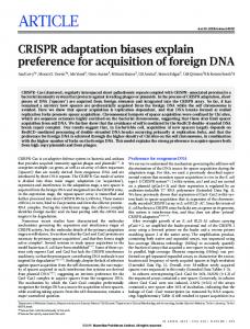
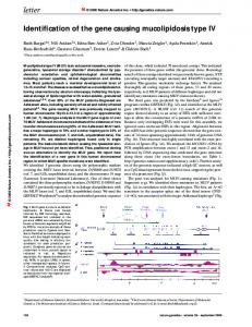
Therefore, is an excellent approximation of for values of not too small (see Fig. 1 for a graphical illustration). As before, we let denote the feature mapping associated with the kernel . The surrogate kernel that we will pick is defined as follows:

(6) is a parameter and is the Gaussian kernel with kernel width . Note that this is a valid kernel by the reverse direction of Theorem 4. is an excellent approxiIf is chosen not too small, then for all , . The reason why we must settle for mation to approximations of the radial kernel, rather than the kernel itself, is the following: for each in the above integral, we construct a . The sursurrogate kernel such that rogate kernel is based on subtracting certain constants from along each dimension, and this cannot be the kernel width done if is larger than those constants. By Fubini’s theorem, we can write (6) as where

3To be precise, the theorem here is a corollary of Schoenberg’s theorem, which discusses necessary and sufficient conditions for k (1; 1) to be positive definite, and Mercer’s theorem (see [8]), which asserts that such a function is a kernel of a valid RKHS.

(8) As before, we let denote the feature mapping associated with this kernel. This is a valid kernel by the reverse direction of Theorem 4. Our algorithm looks exactly like Algorithm 3, only that now we use the new definitions of , above. To state the bound, for some , recall that for any to be the angle between and we define . The bound takes the following form. Theorem 5: Let be the squared loss. For all assume that is perturbed by Gaussian noise with known , and is perturbed by arbitrary indedistribution . Let and pendent noise with 4Note that the scaling factor 1=d is the reasonable one to take, when we assume that the attribute values in the instances are on the order of 2(1).

7916


Fig. 1. Comparison of g (x; x ) (solid line) and k (x; x ) (dashed line) as a function of kx 0 x k, for c = 2 (left) and c = 4 (right). Note that for c = 4, the two graphs are visually indistinguishable.

be fixed. If we run Algorithm 3 with the kernel (7) where , and input parameters

and

then

where and is the feature mapping induced by the kernel (7). The proof of the theorem is provided in Section VIII-C. V. UNKNOWN NOISE DISTRIBUTION In this part of the paper, we turn to study the setting where we wish to learn kernel-based predictors, while having no information about the noise distribution other than an upper bound on its variance. This is relevant in cases where the noise is hard to model, or if it might change in an unexpected or even adversarial manner. Moreover, we provide results with respect to general analytic loss functions, which go beyond the squared loss on which we focused in Section IV. We emphasize that the techniques here are substantially different than those of Section IV, and do not rely on surrogate kernels. Instead, the techniques focus on construction of unbiased gradient estimates directly in the RKHS.

A. Algorithm We present our algorithmic approach in a modular form. We start by introducing the main algorithm, which contains several subroutines. Then we prove our two main results, which bound the regret of the algorithm, the number of queries to the oracle, and the running time for two types of kernels: dot product and Gaussian (our results can be extended to other kernel types as well). In itself, the algorithm is nothing more than a standard onregret line gradient descent algorithm with a standard bound. Thus, most of the proofs are devoted to a detailed discussion of how the subroutines are implemented (including explicit pseudo-code). In this subsection, we describe just one subroutine, based on the techniques discussed in Section III. The other subroutines require a more detailed and technical discussion, and thus their implementation is described as part of the proofs in Section VIII. In any case, the intuition behind the implementations and the techniques used are described in Section III. For the remainder of this subsection, we assume for simplicity that is a classification loss; namely, it can be written as a func. It is not hard to adapt the results below tion of to the case where is a regression loss (where is a function of ). Another simplifying assumption we will make, purely in the interest of clarity, is that the noise will be restricted just to the instance , and not to the target value . In other words, we assume that the learner is given access to , and to an oracle which provides noisy copies of . This does not make our lives easier, since the hard estimation problems relate and not (e.g., estimating in an unbiased to manner, despite the nonlinearity of the feature mapping ). On the other hand, it will help to make our results more transparent, and reduce tedious bookkeeping. At each round, the algorithm below constructs an object (note that it has no relationship which we denote as to used in the previous section). This object has two interpretations here: formally, it is an element of a reproducing kernel Hilbert space (RKHS) corresponding to the kernel we . However, in terms use, and is equal in expectation to


of implementation, it is simply a data structure consisting of a finite set of vectors from . Thus, it can be efficiently stored in memory and handled even for infinite-dimensional RKHS. , has also two interpretations: formally, it Like is an element in the RKHS, as defined in the pseudocode. In terms of implementation, it is defined via the data structures and the values of at round . To apply this hypothesis on a given instance , we compute , where is a subroutine which returns the inner product (a pseudocode is provided as part of the proofs in Section VIII). We start by considering dot-product kernels; that is, kernels that can be written as , where has a Taylor expansion such that for all —see theorem 4.19 in [8]. Our first result shows what regret bound is achievable by the algorithm for any dot-product kernel, as well as characterize the number of oracle queries per instance, and the overall running time of the algorithm. The proof is provided in Section VIII-E. Theorem 6: Assume that the loss function has an analytic for all in its domain, and derivative (assuming it exists). Pick any let dot-product kernel . Finally, assume that for any returned by the oracle at round , for all . Then, for all and , it is possible to implement the subroutines of Algorithm 4 such that: is 1) The expected number of queries to each oracle

7917

Algorithm 4 Kernel Learning Algorithm with Noisy Input : Learning rate sample parameter

, number of rounds

,

: for all

.

for all //

is a data structure which can store a

// variable number of vectors in

Define Receive oracle

and

Let // Get unbiased estimates of

in the RKHS

Let // Get unbiased estimate of Let

// Perform gradient step

Let // Compute squared norm, where returns If

2) The expected running time of the algorithm is

Let

for all

//If squared norm is larger than

3) If we run Algorithm 4 with

where

then

, then project

We note that the distribution of the number of oracle queries can be specified explicitly, and it decays very rapidly—see the proof for details. The parameter is user-defined, and allows one to perform a tradeoff between the number of noisy copies required for each example, and the total number of examples. In other words, the regret bound will be similar whether many noisy measurements are provided on a few examples, or just a few noisy measurements are provided on many different examples. The result pertaining to radial kernels is very similar, and uses essentially the same techniques. For the sake of clarity, we provide a more concrete result which pertains specifically to the most important and popular radial kernel, namely the Gaussian kernel. The proof is provided in Section VIII-F. Theorem 7: Assume that the loss function has an analytic derivative for all in its domain, and let (assuming it exists). Pick any Gaussian for some . Fikernel nally, assume that for any returned by the . Then for all and oracle at round , for all it is possible to implement the subroutines of Algorithm 4 such that

7918


1) The expected number of queries to each oracle

is

2) The expected running time of the algorithm is

3) If we run Algorithm 4 with

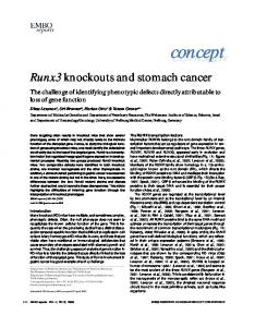
where Fig. 2. Absolute loss, hinge loss, and analytic approximations. For the absolute i 0 y . For the hinge loss, the line represents the loss as a function of h ; loss, the lines represent the loss as a function of y h ; i.

w 9(x) w 9(x)

then

Denote the output of the subroutine above as . Then for any given

As in Theorem 6, note that the number of oracle queries has a fast decaying distribution. Also, note that with Gaussian kernels, is usually chosen to be on the order of the example’s squared norms. Thus, if the noise added to the examples is proportional , and to their original norm, we can assume that thus appearing in the bound is also bounded by a constant. As previously mentioned, most of the subroutines are described in the proofs section, as part of the proof of Theorem 6. Here, we only show how to implement the subroutine, which returns the gradient length estimate . The idea is based on the technique is an unbiased described in Section III-C. We prove that estimate of , and bound . As discussed is analytic and can be written as earlier, we assume that . Subroutine 1 Sample nonnegative integer

in the RKHS

Return

Lemma 4: Assume that returns

and

where the expectation is with respect to the randomness of Subroutine 1. corProof: The result follows from Lemma 1, where responds to the estimator , the function corresponds to , and the random variable corresponds to (where is random and is held fixed). The term Lemma 1 can be upper bounded as

in

B. Loss Function Examples according to

Let // Get unbiased estimate of

it holds that

, and define

, and that for all , .

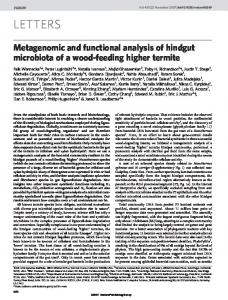
Theorems 6 and 7 both deal with generic loss functions whose derivative can be written as , and the regret . Below, we bounds involve the functions present a few examples of loss functions and their corresponding . As mentioned earlier, while the theorems in the previous subsection are in terms of classification losses (i.e., is a func), virtually identical results can be proven for tion of regression losses (i.e., is a function of ), so we will give examples from both families. Working out the first two examples is straightforward. The proofs of the other two appear in Section VIII-G. The loss functions in the last two examples are illustrated graphically in Fig. 2. Example 1: For the squared loss function, , we have

.


Example 2: For the exponential loss function,

we

have .

Example 3: Recall that the standard absolute loss is defined as . Consider a “smoothed” ab, defined as an antiderivasolute loss function for some (see proof for exact analytic tive of form). Then we have that

Example 4: Recall that the standard hinge loss is defined . Consider as , defined as an ana “smoothed” hinge loss tiderivative of for some (see proof for exact analytic form). Then we have that

For any , the loss function in the last two examples is convex, and, respectively, approximate the absolute loss and the hinge loss arbitrarily well for large enough . Fig. 2 shows these loss functions graphically . Note that need not be large in order to get a good for approximation. Also, we note that both the loss itself and its gradient are computationally easy to evaluate. Finally, we remind the reader that as discussed in Section III-C, performing an unbiased estimate of the gradient for nondifferentiable losses directly (such as the hinge loss or absolute loss) appears to be impossible in general. On the flip side, if one is willing to use a random number of queries with polynomially decaying rather than exponentially-decaying tails, then one can achieve much better sample complexity results, by focusing on loss functions (or approximations thereof) which are only differentiable to a bounded order, rather than fully analytic. This again demonstrates the tradeoff between the number of examples, and the amount of information that needs to be gathered on each example. VI. ARE MULTIPLE NOISY COPIES NECESSARY? The positive results discussed so far are mostly based on getting more than one noisy copy per example. However, one might wonder if this is really necessary. In some applications this is inconvenient, and one would prefer a method which works when just a single noisy copy of each example is made available. Moreover, in the setting of known noise covariance (Section IV-B), for linear predictors and squared loss, we in order to needed just one noisy copy of each example learn. Perhaps a similar result can be obtained even when the noise distribution in unknown?

7919

In this subsection we show that, unfortunately, such a method cannot be found. Specifically, we prove that if the noise distribution is unknown, then under very mild assumptions, no method can achieve sublinear regret, when it has access to just a single (even when is known). On noisy copy of each instance the other hand, for the case of squared loss and linear kernels, we know that we can learn based on two noisy copies of each instance (see Section IV-A). So without further assumptions, the lower bound that we prove here is indeed tight. It is an interesting open problem to show improved lower bounds when nonlinear kernels are used, or when the loss function is more complex. Theorem 8: Let be a compact convex subset of , and let satisfies the following: (1) it is bounded from . For any below; (2) it is differentiable at 0 with and is allearning algorithm which selects hypotheses from lowed access to a single noisy copy of the instance at each round , there exists a strategy for the adversary such that the sequence of predictors output by the algorithm satisfies

with probability 1. Note that condition (1) is satisfied by virtually any loss function other than the linear loss, while condition (2) is satisfied by most regression losses, and by all classification calibrated losses, which include all reasonable losses for classification (see [23]). The intuition of the proof is very simple: the adversary chooses beforehand whether the examples are drawn i.i.d. from a distribution , and then perturbed by noise, or drawn without adding noise. i.i.d. from some other distribution The distributions , and the noise are designed so that the examples observed by the learner are distributed in the same way irrespective of which of the two sampling strategies the adversary chooses. Therefore, it is impossible for the learner accessing a single copy of each instance to be statistically consistent with respect to both distributions simultaneously. As a result, the adversary can always choose a distribution on which the algorithm will be inconsistent, leading to constant regret. To prove the theorem, we use a more general result which leads to nonvanishing regret, and then show that under the assumptions of Theorem 8, the result holds. The proof of the result is given in Section VIII-I. be a compact convex subset of and Theorem 9: Let pick any learning algorithm which selects hypotheses from and is allowed access to a single noisy copy of the instance at each round . If there exists a distribution over a compact subset of such that

(9)

7920


are disjoint, then there exists a strategy for the adversary such of predictors output by the that the sequence algorithm satisfies

VIII. PROOFS A. Proof of Theorem 1 First, we use the following lemma that can be easily adapted from [11].

with probability 1. Another way to phrase this theorem is that the regret cannot vanish, if given examples sampled i.i.d. from a distribution, the learning problem is more complicated than just finding the mean of the data. Indeed, the adversary’s strategy we choose later on is simply drawing and presenting examples from such a distribution. Below, we sketch how we use Theorem 9 in order to prove Theorem 8. A full proof is provided in Section VIII-H. We construct a very simple one-dimensional distribution, which satisfies the conditions of Theorem 9: it is simply , where is the vector the uniform distribution on . Thus, it is enough to show that

Lemma 5: Let be a sequence of vectors. Let and for let , where is the pro. Then, jection operator on an origin-centered ball of radius we have for all such that

Applying Lemma 5 with obtain

as defined in Lemma 2, we

Taking expectation of both sides and using again Lemma 2, we obtain that

(10) are disjoint, for some appropriately chosen . Assuming the contrary, then under the assumptions on , we show that the first set in (10) is inside a bounded ball around the origin, in a way , no matter how large it is. Thus, if which is independent of we pick to be large enough, and assume that the two sets in (10) are not disjoint, then there must be some such that both and have a subgradient of zero at . However, this can be shown to contradict the assumptions on , leading to the desired result.

Now, using convexity we get that

which gives

Picking

as in the theorem statement concludes our proof.

B. Proof of Theorem 3 VII. CONCLUSIONS AND FUTURE WORK We have investigated the problem of learning, in an online fashion, linear and kernel-based predictors when the observed examples are corrupted by noise. We have shown bounds on the expected regret of learning algorithms under various assumptions on the noise distribution and the loss function (squared loss, analytic losses). A key ingredient of our results is the derivation of unbiased estimates for the loss gradients based on the possibility of obtaining a small but random number of independent copies of each noisy example. We also show that accessing more than one copy of each noisy example is a necessary condition for learning with sublinear regret. There are several interesting research directions worth pursuing in the noisy learning framework introduced here. For instance, doing away with unbiasedness, which could lead to the design of estimators that are applicable to more types of loss functions, for which unbiased estimators may not even exist. Biased estimates may also help in designing improved estimates for kernel learning when the noise distribution is known, but not necessarily Gaussian. Another open question is whether our lower bound (Theorem 8) can be improved when nonlinear kernels are used.

To prove the theorem, we will need a few auxiliary lemmas. In particular, Lemma 6 is a key technical lemma, which will prove , , crucial in connecting the RKHS with respect to and the RKHS with respect to , . Lemma 8 connects between the norms of elements in the two RKHS’s. To state the lemmas and proofs conveniently, recall the shorthand

Lemma 6: For any , , if we let where is a Gaussian random vector with covariance matrix , then it holds that

Proof: The expectation in the lemma can be written as

(11)


7921

A purely technical integration exercise reveals that each element in this product equals . Therefore, (11) equals

which is exactly Lemma 7: Let RKHS. Let scalars, such that it holds that

right-hand side (RHS) of the inequality above, we get an upper bound of the form

. denote a feature mapping to an arbitrary be vectors in , and for some . Then

where we used the fact that . A straightforward upper bounding leads to the lemma statement. The following lemma is basically a corollary of Lemma 7. be vectors in , and Lemma 8: Let scalars, such that . is an element in the RKHS with respect to Then , whose norm squared is at most

where

is the angle between and in the RKHS (or if one of these elements is zero). We remark that this bound is designed for readability—it is not the tightest upper bound possible. or Proof: The bound trivially holds if are zero, so we will assume w.l.o.g. that they are both nonzero. To simplify notation, let

Here,

is the angle between in the RKHS (or elements is zero). and Proof: Picking some lemma statement, we have

and if one of the as in the

(13) where the last transition is by the fact that is always positive. , , it holds for any , that Now, by definition of

and notice that fact that

. By the cosine theorem and the , we have that which is at most

Solving for and taking the larger root in the resulting quadratic equation, we have that

. Therefore, we can upper bound (13) by

The lemma follows by noting that according to Lemma 7

(12) (it is easy to verify that the term in the squared root is always nonnegative). Therefore

From straightforward geometric arguments, we must have (this is the same reason the term in the squared root in (12) is nonnegative). Plugging this into the

With these lemmas in hand, we are now ready to prove the main theorem. denote the value of in To make the proof clearer, let algorithm 3 at the beginning of round .

7922


The first step of the proof consists of applying Lemma 5, since our algorithm follows the protocol outlined in that lemma, using kernels. We therefore have that for any in the RKHS corresponding to , such that , it holds that

Plugging this back into (15), and choosing orem’s statement, we finally get

as in the the-

(16) (14) In particular, consider statement, and define

We now turn to analyze the more interesting LHS of (16). The LHS of (16) can be written as

from the theorem’s (17) In order to analyze the first sum inside the expectation, recall can be written as . Therefore, we have that that

This is an element in the RKHS corresponding to , but it shares the same set of weights as , which is an element in the . Since , it follows RKHS corresponding to from Lemma 8 and the definition of that . Therefore, (14) applies, and we get where the last transition is by the fact that , , are mutuconally independent, and therefore is independent of . ditioned on We now make two crucial observations, which are really the heart of our proof: First, by Lemma 6, we have that This inequality holds for any . In particular, it will remain valid if we take expectations of both sides with respect to the Gaussian noise injected into the unperturbed data Second, using Lemma 6 in a similar manner, we also have

(15) Starting with the RHS, we note that by definition of from the algorithm’s pseudocode, and the fact that

Define this expression as . Notice that it is exactly the gradient of with respect to . As a result of these two observations, we get overall that

by definition of the kernel in (5) (18) Moving to the second sum in the LHS of (17), recall that there such that . exist some Therefore

As before, we have by Lemma 6 that , and that is conditionally independent with


7923

expected value . Substituting this into the expression above, we get that it is equal to

Also, by a Taylor expansion of the log function, and using the by the assumption that , we get fact that

(21)

Combining this and (18), and summing over , we get that Plugging this into (20), we get the upper bound

(19) in the Remarkably, this equation links between classifiers , and the classifiers in another RKHS corresponding to . RKHS, corresponding to Substituting (19) into (16), we get that

, if we let where Lemma 10: For any , is a Gaussian random vector with covariance matrix , then it holds that

Proof: On one hand, based on the definition of equals can be verified that

in (7), it

(22) Now, since convex function of , and since we can lower bound the LHS as

is the gradient at

is a ,

On the other hand, using the proof of Lemma 6 and Fubini’s theorem, the expectation in the lemma can be written as

from which the theorem follows. C. Proof of Theorem 5 The proof follows the same lines as the proof of Theorem 3 in the previous subsection. The changes mostly have to do with the auxiliary lemmas, which we present below. The proof of the theorem itself is virtually identical to the one of Theorem 3, and is thus skipped. The auxiliary lemmas below modify the parallel lemmas in Section VIII-B, based on the new definitions of the feature mapping and the surrogate feature mapping . But before that, we for begin with a lemma which explicitly upper bounds any . With Gaussian kernels, this was trivial, but now we need to work a bit harder. Lemma 9: For any vector

Lemma 11: Let be vectors in , and scalars, such that . Then is an element in the RKHS with respect to , whose norm squared is at most

, we have Here,

is the angle between in the RKHS (or elements is zero). and Proof: Picking some lemma statement, we have

Proof: By (8)

(20)

and is one of the as in the

(23)

7924


Now, by definition of in (8), and the representation of as in (22), it holds for any , that equals

Here the expectation is with respect to both the randomness of the oracles and of the algorithm throughout its run. Proof: Our algorithm corresponds to Zinkevich’s online gradient descent algorithm [11] in a finite horizon setting, where we assume the sequence of examples is , the cost function is linear, and . By a straightforward the learning rate at round is adaptation of the standard regret bound for that algorithm (see [11]), we have that for any such that

where the last transition can be verified as in (21). Therefore, we can upper bound (23) by

We now take expectation of both sides in the inequality above. The expectation of the RHS is simply

The lemma follows by noting that

which according to Lemma 7 is at most

.

As to the LHS, note that

D. Preliminary Result for Proving Theorem 6 and Theorem 7 To prove Theorem 6 and Theorem 7, we need a theorem which basically states that if all subroutines in algorithm 4 behave as they should, then one can achieve an regret bound. This is provided in the following theorem, which is an adaptation of a standard result of online convex optimization (see, e.g., [11]). Theorem 10: Assume the following conditions hold with respect to Algorithm 4: and are independent of each other (as 1) For all , random variables induced by the randomness of Algorithm and for . 4) as well as independent of any , and there exists a constant 2) For all , such that

3) For all , such that constant 4) For any pair of instances ,

If Algorithm 4 is run with

Also

Plugging in these expectations and choosing as in the statement of the theorem, we get that for any such that

, and there exists a .

, then

To get the theorem, we note that by convexity of , the LHS above can be lower bounded by


E. Proof of Theorem 6 Based on the preliminary result of Section VIII-D, we present in this subsection the proof of Theorem 6. We first show how to implement the subroutines of Algorithm 4, and prove the relevant results on their behavior. Then, we prove the theorem itself. corWe start by constructing an explicit feature mapping responding to the RKHS induced by our kernel. For any , , we have that

This suggests the following feature representation: for any , returns an infinite-dimensional vector, indexed by and , with the entry corresponding being . The inner product to and is similar to a standard dot product between between two vectors, and by the derivation above equals as required. We now use a slightly more elaborate variant of our unbiased . estimate technique, to derive an unbiased estimate of First, we sample according to . for times to get Then, we query the oracle for , and formally define as

7925

where we recall that defines the kernel by . Proof: The first part of the lemma follows from the discussion above. As to the second part, note that by (24)

where the second-to-last step used the fact that .

for all

Of course, explicitly storing as defined above is infeasible, since the number of entries is huge. Fortunately, this is not . The representaneeded: we just need to store tion above is used implicitly when we calculate inner products and other elements in the RKHS. We note that between while is a random quantity which might be unbounded, its distribution decays exponentially fast, so the number of vectors to store is essentially bounded. After the discussion above, the pseudocode for below should be self-explanatory. Subroutine 2

(24) where represents the unit vector in the direction inas explained above. Since the oracle dexed by queries are i.i.d., the expectation of this expression is

Sample nonnegative integer

Query

for

Return

according to

times to get as

.

We now turn to the subroutine , which given two ele, in the RKHS, returns their inner product. ments which is exactly . We formalize the needed properties of in the following lemma.

Subroutine 3

Lemma 12: Assuming sion above, it holds that over, if the noisy samples , then

Let

is constructed as in the discusfor any . Morereturned by the oracle satisfy

be the vectors comprising

Let If

be the vectors comprising return 0, else return

Lemma 13:

returns

.

7926


Proof: Using the formal representation of , in (24), we have that is 0 whenever (because then these two elements are composed of different unit vectors with respect to an orthogonal basis). Otherwise, we have that

Since Algorithm 4 at each of rounds calls once, once, for times, other operations, we get that the overall runand performs time is

Since

which is exactly what the algorithm returns, hence the lemma follows. As discussed in the main text, in order to apply the learned predictor on a new given instance , we present another subroutine , which calculates the inner product . The pseudocode is very similar to the subroutine, and the proof of correctness is essentially the same. Subroutine 4 Let


Return We are now ready to prove Theorem 6. First, regarding the expected number of queries, notice that to run Algorithm and 4, we invoke once at round . uses a random number of queries distributed as , and invokes a random . number of times, distributed as The total number of queries is therefore , where for all are i.i.d. copies of . The expected value of this expression, using a standard result on the expected value of a sum of a random number of independent random variables, is , or . equal to In terms of running time, we note that the expected running time of is , this because it performs multiplications of inner products, each one with running , and . The expected running time of time is . The expected running time of is

, we can upper bound this by

The regret bound in the theorem follows from Theorem 10, with the expressions for constants following from Lemma 4, Lemma 12, and Lemma 13. F. Proof of Theorem 7 The proof here is based on the preliminary result of Section VIII-D. The analysis in the Gaussian kernel case is rather similar to the one for inner product kernel case (in Section VIII-E), with some technical changes. Thus, we provide the proof here mostly for completeness. We start by constructing an explicit feature mapping corresponding to the RKHS induced by our kernel. For any , , we have that

This suggests the following feature representation: for any , returns an infinite-dimensional vector, indexed by and , with the entry corresponding being . The inner to and is similar to a standard inner product between product between two vectors, and by the derivation above as required. equals is the folThe idea of deriving an unbiased estimate of , independently according to lowing: first, we sample . Then, we query


the oracle for for and formally define

times to get

7927

,

as

Proof: The first part of the lemma follows from the discussion above. As to the second part, note that by (25), we have that equals

(25) represents the unit vector in the direction where as explained above. Since the oracle indexed by calls are i.i.d., it is not hard to verify that the expectation of the expression above is

The expectation of this expression over

as defined above. in memory, we simply keep and . The representation above is used implicand other itly when we calculate inner products between elements in the RKHS, via the subroutine Prod. We formalize in the following lemma. the needed properties of

,

is equal to

which is exactly To actually store

Lemma 14: Assuming the construction of as in the disfor all . Morecussion above, it holds that returned by the oracle satisfies over, if the noisy sample , then

After

the

discussion above, the pseudocode below should be self-explanatory.

Subroutine 5 Sample

according to

Sample

according to

Query Return

for

times to get as

.

for

7928


We now turn to the subroutine given the two elements inner product.

(Subroutine 10), which in the RKHS, returns their

G. Proof of Examples 3 and 4

Subroutine 6 be the vectors comprising

Let Let If

The regret bound in the theorem follows from Theorem 10, with the expressions for constants following from Lemma 4, Lemma 14, and Lemma 15.

be the vectors comprising return 0, else return

in order to Examples 3 and 4 use the error function construct analytic approximations of the hinge loss and the absolute loss (see Fig. 2). The error function is useful for our purposes, since it is analytic in all of , and smoothly interpolates for and 1 for . Thus, it can be used between to approximate derivative of losses which are piecewise linear, and the absolute such as the hinge loss . loss To approximate the absolute loss, we use the antiderivative . This function represents an analytic upper bound on of the absolute loss, which becomes tighter as increases. It can be verified that the antiderivative (with the constant free parameter fixed so the function has the desired behavior) is

The proof of the following lemma is a straightforward algebraic exercise, similar to the proof of Lemma 13. Lemma 15: returns . As described in the main text, when we wish to apply our learned predictor on a given instance , we also need a subroutine to compute , where is an explicitly given vector. The pseudocode is described in Subroutine 11. It is very similar to Subroutine 10, and the proof is essentially the same.

While this loss function may seem to have slightly complex form, we note that our algorithm only needs to calculate the derivative of this loss function at various points (namely for various values of ), which can be easily done. By a Taylor expansion of the error function, we have that

Subroutine 7 Therefore, Let

in this case is at most


Return

We are now ready to prove Theorem 7. First, regarding the expected number of queries, notice that to run Algorithm and 4, we invoke once at round . uses a random number of queries, where , are independent and . distributed as invokes a random number of times, where . The , total number of queries is therefore , are i.i.d. copies of , , respectively. The where expected value of this expression, using a standard result on the expected value of a sum of a random number of random , or variables, is equal to . In terms of running time, the analysis is completely identical to the one performed in the proof of Theorem 6, and the expected running time is the same up to constants.

We now turn to deal with Example 4. This time, we use the antiderivative of . This function smoothly infor and 0 for . Therefore, terpolates between its antiderivative with respect to represents an analytic upper bound on the hinge loss, which becomes tighter as increases. It can be verified that the antiderivative (with the constant free parameter fixed so the function has the desired behavior) is

By a Taylor expansion of the error function, we have that

Thus,

in this case can be upper bounded by


H. Proof of Theorem 8

7929

I. Proof of Theorem 9

to be specified later. Let Fix a large enough and let to be the uniform distribution on . To prove the result then we just need to show that and (26) . are disjoint, for some appropriately chosen First, we show that the first set above is a subset of for some fixed which does not depend on . looks We do a case-by-case analysis, depending on how like. monotonically increases in . Impossible by as1) sumption (2). monotonically decreases in . First, recall that 2) since is convex, it is differentiable almost anywhere, and its derivative is monotonically increasing. is convex and bounded from below, Now, since must tend to 0 as (wherever is differentiable, which is almost everywhere by convexity). is upper bounded Moreover, by assumption (2), . As a reby a strictly negative constant for any , which equals sult, the gradient of , must be positive for large enough , and negative for large enough , so the are in some bounded minimizers of subset of . 3) There is some such that monotonically deand monotonically increases in . creases in or in , we If the function is constant in are back to one of the two previous cases. Otherwise, by , we must have some , , convexity of , such that is strictly decreasing at , and . In that case, it is not hard to strictly increasing at must be strictly increasing see that for any , and strictly decreasing for . So again, the minimizers of any are in some bounded subset of . We are now ready to show that the two sets in (26) must be dislarge enough so that the first set in joint. Suppose we pick . Assume on the con(26) is strictly inside , which belongs to both trary that there is some , sets in (26). By assumption (2) and the fact that minimizes , we may assume . Therefore, as , where is the (closed and well as convex) subgradient set of a convex function . By subgradient and calculus, this means there is some such that . This implies that . Now, suppose that . This . But then is strictly would mean that , and in particular , decreasing at contradicting the assumption that minimizes . So we . Moreover, must have (because minimizes and ). Since the subgra. dient set is closed and convex, it follows that Therefore, both and minimize . But this means that , in contradiction to assumption (2).

Let be a distribution which satisfies (9). The idea of the proof is that the learner cannot know if is the real distribution (on which regret is measured) or the distribution which includes noise. Specifically, consider the following two adversary strategies: 1) At each round, draw an example from , and present it to the learner (with the label 1) without adding noise. , add to it zero-mean 2) At each round, pick the example , where is distributed noise sampled from according to , and present the noisy example (with the label 1) to the learner. In both cases the examples presented to a learner appear to come from the same distribution . Hence, any learner observing one copy of each example cannot know which of the two strategies is played by the adversary. Since (9) implies that the set of optimal learner strategies for each of the two adversary strategies are disjoint, by picking an appropriate strategy the adversary can force a constant regret. To formalize this argument, fix any learning algorithm that be the observes one copy of each example and let sequence of generated predictors. Then it is sufficient to show that at least one of the following two holds

(27)

(28) with probability 1, where in both cases the expectation is with respect to and “w.p. 1” refers to the randomness of the noise. First note that (27) is implied by

(29) is compact, is assumed to be with probability 1. Since supported on a compact subset, and is convex and hence is almost surely bounded. So by continuous, then Azuma’s inequality

is finite for all , where the expectation is conditioned on the randomness in the previous rounds. Letting (which belongs to for all since it is a convex set), we have

7930


where the first inequality holds with probability 1 as by the Borel-Cantelli lemma, and the second one holds for every because is convex. Similarly,

Hence (28)–(29) are obtained if we show that no single sequence simultaneously satisfies of predictors

known to the learner, and at each round provides the example . It is easy to verify that (31) in this case equals

Recall that the learner chooses before is revealed. Therefore, if the noise which leads to has positive variance, it will such that generally be impossible for the learner to choose is arbitrarily close to 1. Therefore, the equation above cannot grow sublinearly with .

(30) where

ACKNOWLEDGMENT The authors would like to thank A. Argyriou for turning our attention to Schoenberg’s theorem and its applicability in our setting. This publication only reflects the authors’ views.

and

REFERENCES Suppose on the contrary that there was such a sequence. for all , and is compact, the sequence Since has at least a cluster point . Moreover, it is easy to verify that the functions and are continuous. is continuous by convexity of and Indeed, is continuous by the compactness assumptions. is also a cluster point Hence, any cluster point of of both and . Since , by construction, and nor for we are assuming that neither . any cluster point , we must have belongs to both sets appearing in (9), But this means that in contradiction to the assumption they are disjoint. Thus, no sequence of predictors satisfies (30), as desired. APPENDIX ALTERNATIVE NOTIONS OF REGRET In the online setting, one may consider notions of regret other than (1). One choice is

but this is too easy, as it reduces to standard online learning with respect to examples which happen to be noisy. Another kind of regret we may want to minimize is (31) This is the kind of regret which is relevant for actually predicting the values well based on the noisy instances. Unfortunately, in general this is too much to hope for. To see why, , and assume we deal with a linear kernel (so that . Now, suppose that the assume in , which might be even adversary picks some

[1] S. Chawla, C. Dwork, F. McSherry, A. Smith, and H. Wee, “Toward privacy in public databases,” in Proc. Theory of Cryptogr. Conf. (TCC), LNCS, 2005, vol. 2. [2] D. Nettleton, A. Orriols-Puig, and A. Fornells, “A study of the effect of different types of noise on the precision of supervised learning techniques,” Artif. Intell. Rev., 2010. [3] N. Bshouty, J. Jackson, and C. Tamon, “Uniform-distribution attribute noise learnability,” Inf. Computat., vol. 187, no. 2, pp. 277–290, 2003. [4] S. Goldman and R. Sloan, “Can pac learning algorithms tolerate random attribute noise?,” Algorithmica, vol. 14, no. 1, pp. 70–84, 1995. [5] M. Kearns and M. Li, “Learning in the presence of malicious errors,” SIAM J. Comput., vol. 22, no. 4, pp. 807–837, 1993. [6] N. Cesa-Bianchi, E. Dichterman, P. Fischer, E. Shamir, and H. Simon, “Sample-efficient strategies for learning in the presence of noise,” J. ACM, vol. 46, no. 5, pp. 684–719, 1999. [7] N. Littlestone, “Redundant noisy attributes, attribute errors, and linear threshold learning using Winnow,” in Proc. COLT, 1991, pp. 147–156. [8] B. Schölkopf and A. Smola, Learning with Kernels. Cambridge: MIT Press, 2002. [9] N. Cesa-Bianchi, A. Conconi, and C. Gentile, “On the generalization ability of on-line learning algorithms,” IEEE Trans. Inf. Theory, vol. 50, no. 9, pp. 2050–2057, Sep. 2004. [10] I. Steinwart and A. Christmann, Support Vector Machines. New York: Springer, 2008. [11] M. Zinkevich, “Online convex programming and generalized infinitesimal gradient ascent,” in Proc. ICML, 2003, pp. 928–936. [12] N. Cesa-Bianchi and G. Lugosi, Prediction, Learning, and Games. Cambridge, U.K.: Cambridge Univ. Press, 2006. [13] A. Flaxman, A. Kalai, and H. McMahan, “Online convex optimization in the bandit setting: Gradient descent without a gradient,” in Proc. SODA, 2005, pp. 385–394. [14] J. Abernethy, E. Hazan, and A. Rakhlin, “Competing in the dark: An efficient algorithm for bandit linear optimization,” in COLT, 2008, pp. 263–274. [15] L. Paninski, “Estimation of entropy and mutual information,” Neural Computat., vol. 15, no. 6, pp. 1191–1253, 2003. [16] R. Singh, “Existence of unbiased estimates,” Sankhy¯a: The Indian J. Statist., vol. 26, no. 1, pp. 93–96, 1964. [17] S. Bhandari and A. Bose, “Existence of unbiased estimators in sequential binomial experiments,” Sankhy¯a: The Indian J. Statist., vol. 52, no. 1, pp. 127–130, 1990. [18] I. Schoenberg, “Metric spaces and completely monotone functions,” Ann. Math., vol. 39, no. 4, pp. 811–841, Oct. 1938. [19] P. Ressel, “A short proof of Schoenberg’s theorem,” Proc. AMS, vol. 57, no. 1, pp. 66–68, May 1976. [20] C. Micchelli, Y. Xu, and H. Zhang, “Universal kernels,” J. Mach. Learn. Res., vol. 7, pp. 2651–2667, 2006.


[21] C. Scovel, D. Hush, I. Steinwart, and J. Theiler, Radial Kernels and Their Reproducing Kernel Hilbert Spaces Los Alamos Nat. Lab., 2010, Tech. Rep. LA-UR-09-01900. [22] W. Rudin, Fourier Analysis on Groups (reprint edition). New York: Wiley Classics Library, 1994. [23] P. Bartlett, M. Jordan, and J. McAuliffe, “Convexity, classification and risk bounds,” J. Amer. Statist. Assoc., vol. 101, no. 473, pp. 138–156, Mar. 2006. Nicoló Cesa-Bianchi is professor of Computer Science at the University of Milano, Italy. His main research interests include statistical learning theory, game-theoretic learning, and pattern analysis. He is coauthor, with Gabor Lugosi, of the monography “Prediction, Learning, and Games” (Cambridge University Press, 2006). Dr. Cesa-Bianchi was President of the Association for Computational Learning (2006–2009). He is a member of the steering committee of the EC-funded Network of Excellence PASCAL2, action editor for the IEEE TRANSACTIONS ON INFORMATION THEORY and for the Journal of Machine Learning Research. He is a recipient of a Google Research Award (2010).

7931

Shai Shalev-Shwartz is on the faculty of the Department of Computer Science and Engineering, The Hebrew University of Jerusalem, Israel. He is interested in learning theory, online prediction, optimization, and practical algorithms.

Ohad Shamir received the Ph.D. degree from the Department of Computer Science and Engineering, The Hebrew University of Jerusalem. He is a Postdoctoral Researcher at Microsoft Research New England, Cambridge, MA. He is broadly interested in statistical and online machine learning, with emphasis on novel algorithms which combine practical applicability and theoretical insight.

Online Learning of Noisy Data - Weizmann Institute of Science

Online Learning of Noisy Data - Weizmann Institute of Science

Suggest Documents

ARTICLE - Weizmann Institute of Science

concept - Weizmann Institute of Science

cadherins - Weizmann Institute of Science

Acetylcholinesterase - Weizmann Institute of Science

Untitled - Weizmann Institute of Science

Intermittency - Weizmann Institute of Science

TM7SF3 - Weizmann Institute of Science

review - Weizmann Institute of Science

letter - Weizmann Institute of Science

Untitled - Weizmann Institute of Science

INTRODUCTION - Weizmann Institute of Science

nojirimycin - Weizmann Institute of Science

pyruvate - Weizmann Institute of Science

letters - Weizmann Institute of Science

Untitled - Weizmann Institute of Science

letter - Weizmann Institute of Science

["a: - Weizmann Institute of Science

editorial - Weizmann Institute of Science

Online Learning of Noisy Data with Kernels

Table of Contents - Weizmann Institute of Science

Detecting Faint Curved Edges in Noisy Images - Weizmann Institute of

J Neuroimmunol 2000 - Weizmann Institute of Science

Author's personal copy - Weizmann Institute of Science

electronic reprint - Weizmann Institute of Science