to develop a power-aware approach to routing messages in such a ..... left figure gives the network; the center one is the route for ... We call this path the max-.
Online Power-aware Routing in Wireless Ad-hoc Networks Qun Li, Javed Aslam, Daniela Rus Department of Computer Science Dartmouth College Hanover, NH 03755 {liqun, jaa, rus}@cs.dartmouth.edu
Card
ABSTRACT This paper discusses online power-aware routing in large wireless ad-hoc networks for applications where the message sequence is not known. We seek to optimize the lifetime of the network. We show that online power-aware routing does not have a constant competitive ratio to the off-line optimal algorithm. We develop an approximation algorithm called max-min zPmin that has a good empirical competitive ratio. To ensure scalability, we introduce a second online algorithm for power-aware routing. This hierarchical algorithm is called zone-based routing. Our experiments show that its performance is quite good.
1.
RangeLAN2-7410 WaveLAN(11Mbps) Smart Spread
Tr mA 265 284 150
Rv mA 130 190 80
Idle mA n/a 156 n/a
Slp mA 2 10 5
Power Sup. V 5 4.74 5
Table 1: Power Consumption Comparison among Different Wireless LAN Cards ([21, 10, 32]). For RangeLAN2, the power consumption for doze mode (which is claimed to be network aware) is 5mA. The last one is Smart Spread Spectrum of Adcon Telemetry.
INTRODUCTION
The proliferation of low-power analog and digital electronics has created huge opportunities for the field of wireless computing. It is now possible to deploy hundreds of devices of low computation, communication and battery power. They can create ad-hoc networks and be used as distributed sensors to monitor large geographical areas, as communication enablers for field operations, or as grids of computation. These applications require great care in the utilization of power. The power level is provided by batteries and thus it is finite. Every message sent and every computation performed drains the battery.
the power utilized for the transmission of a message; (2) the power utilized for the reception of a message; and (3) the power utilized while the system is idle. Table 1 lists power consumption numbers for several wireless cards. This suggests two complementary levels at which power consumption can be optimized: (1) minimizing power consumption during the idle time and (2) minimizing power consumption during communication. In this paper we focus only on issues related to minimizing power consumption during communication that is, while the system is transmitting and receiving messages. We believe that efficient message routing algorithms, coupled with good solutions for optimizing power consumption during the idle time such as those proposed by [33, 4] will lead to effective power management in wireless ad-hoc networks, especially for a sparsely deployed network.
In this paper we examine a class of algorithms for routing messages in wireless networks subject to power constraints and optimizations. We envision a large ad-hoc network consisting of thousands of computers such as a sensor network distributed over a large geographical area. Clearly this type of network has a high degree of redundancy. We would like to develop a power-aware approach to routing messages in such a system that is fast, scalable, and is online in that it does not know ahead of time the sequence of messages that has to be routed over the network.
Several metrics can be used to optimize power-routing for a sequence of messages. Minimizing the energy consumed for each message is an obvious solution that optimizes locally the power consumption. Other useful metrics include minimizing the variance in each computer power level, minimizing the ratio of cost/packet, and minimizing the maximum node cost. A drawback of these metrics is that they focus on individual nodes in the system instead of the system as a whole. Therefore, routing messages according to them might quickly lead to a system in which nodes have high residual power but the system is not connected because some critical nodes have been depleted of power. We choose to focus on a global metric by maximizing the lifetime of the network. We model this as the time to the earliest time a message cannot be sent. This metric is very useful for ad-hoc networks where each message is important and the networks are sparsely deployed.
The power consumption of each node in an ad-hoc wireless system can be divided according to functionality into: (1) Permission to make digital or hard copies of part or all of this work or personal or classroom use is granted without fee provided that copies are not made or distributed for profit or commercial advantage and that copies bear this notice and the full citation on the first page. To copy otherwise, to republish, to post on servers, or to redistribute to lists, requires prior specific permission and/or a fee. ACM SIGMOBILE 7/01 Rome, Italy © 2001 ACM ISBN 1-58113-422-3/01/07…$5.OO
97
In this paper we show that the online power-aware message routing problem is very hard (Section 3). This problem does not have a constant competitive ratio to the off-line optimal algorithm that knows the message sequence. Guided by this theoretical result, we propose an online approximation algorithm for power-aware message routing that optimizes the lifetime of the network and examine its bounds (Section 4). Our algorithm, called the max-min zPmin algorithm, combines the benefits of selecting the path with the minimum power consumption and the path that maximizes the minimal residual power in the nodes of the network. Despite the discouraging theoretical result concerning the competitive ratio for online routing, we show that the max-min zPmin algorithm has a good competitive ratio in practice, approaching the performance of the optimal off-line routing algorithm under realistic conditions.
the short path at the beginning, has inspired the approach described in this paper. We also use the same formula to describe the residual power fraction. In [12], Gupta and Kumar discussed the critical power at which a node needs to transmit in order to ensure the network is connected. Energy efficient MAC layer protocols can be found in [7, 6]. The work presented in this paper is different from these previous results in that we develop online, hierarchical, and scalable algorithms that do not rely on knowing the message rate and optimize the lifetime of the network. A recent and very important body of work concerns optimizing power consumption during idle time rather than during the time of communicating messages [33, 4]. This work is complementary to the results presented in this paper. Combined, efficient ways for dealing with idle time and with communication can lead to powerful power management solutions.
Our proposed max-min zPmin algorithm requires information about the power level of each computer in the network. Knowing this information accurately is not a problem in small networks. However, for large networks it is difficult to aggregate and maintain this information. This makes it hard to implement the max-min zPmin algorithm for large networks. Instead, we propose another online algorithm called zone-based routing that relies on max-min zPmin and is scalable (Section 5). Our experiments show that the performance of zone-base routing is very close to the performance of max-min zPmin with respect to optimizing the lifetime of the network.
Related results in sensor networks include [27, 1, 15, 9, 14, 5]. The high-level vision of wireless sensor networks was introduced in [27, 1]. Achieving energy-efficient communication is an important issue in sensor network design. Using directed diffusion for sensor coordination is described in [15, 9]. In [14] a low-energy adaptive protocol that uses data fusion is proposed for sensor networks. Our approach is different than this previous work in that we consider message routing in sensor networks and our solution does not require to know or aggregate the data transmitted.
Zone-base routing is a hierarchical approach where the area covered by the (sensor) network is divided into a small number of zones. Each zone has many nodes and thus a lot of redundancy in routing a message through it. To send a message across the entire area we find a “global” path from zone to zone and give each zone control over how to route the message within itself. Thus, zone-based power-aware routing consists of (1) an algorithm for estimating the power level of each zone; (2) an algorithm computing a path for each message across zones; and (3) an algorithm for computing the best path for the message within each zone (with respect to the power lifetime of the zone.)
2.
3.
FORMULATION OF POWER-AWARE ROUTING 3.1 The Model Power consumption in ad-hoc networks can be divided into two parts: (1) the idle mode and (2) the transmit/receive mode. The nodes in the network are either in idle mode or in transmit/receive mode at all time. The idle mode corresponds to a baseline power consumption. Optimizing this mode is the focus of [33, 4]. We instead focus on studying and optimizing the transmit/receive mode. When a message is routed through the system, all the nodes with the exception of the source and destination receives a message and then immediately relay it. Because of this, we can view the power consumption at each node as an aggregate between transit and receive powers which we will model as one parameter as described below.
RELATED WORK
We are inspired by exciting recent results in ad-hoc networks and in sensor networks. Most previous research on ad-hoc network routing [17, 13, 23, 24, 26, 30, 19, 18] focused on the protocol design and performance evaluation in terms of the message overhead and loss rate. To improve the scalability of routing algorithms for large networks, many hierarchical routing methods have been proposed in [20, 8, 22, 2, 11, 28]. In [25, 16], zones, which are the route maintenance units, are used to find the routes. This previous work focused on how to find the correct route efficiently, but did not consider optimizing power while sending messages.
More specifically, we assume an ad-hoc network that can be represented by a weighted graph G(V, E). The vertices of the graph correspond to computers in the network. They have weights that correspond to the computer’s power level. The edges in the graph correspond to pairs of computers that are in communication range. Each weight between nodes is the power cost of sending a unit message1 between the two nodes.
Singh et al. [31] proposed power-aware routing and discussed different metrics in power-aware routing. Some of the ideas in this paper are extensions of what that paper proposed. Minimal energy consumption was used in [29]. Chang and Tassiulas [3] also proposed maximizing the lifetime of a network when the message rate is known. Their main idea, namely to avoid using low power nodes and choose
Suppose a host needs power e to transmit a message to another host who is d distance away. We use the model of [3, 14] to compute the power consumption for sending this 1
Without loss of generality, we assume that all the messages are unit messages. Longer messages can be expressed as sequences of unit messages.
98
��������� ��������� ��������� ��������� ����������� �������������� ����������� ����������� ����������� ����������� ����������� ������� ��� ��� ��� ��� ��� ���� ����������������� ��������� ��������� ��������� ��������� ��������� ��������� ��������� ��������� ��������� ����������� ���������� ������ ���������� ���������������� ���������������� ���������������� ���������������� ���������������� ������������ ��������������� ��� ���������� ������ ��� ���������� ������ ��� ���������� ������ ��� ���������� ������ ��� �������� ���������������� �� �� ������������������ ������������������ ������������������ ������������������ ������������������ �� ���������������� �
������������ ��� ��������� ��� ��������� ��� ��������� ��� ��������� ����� ������������� �� ������������ ������������ ������������ ������������ ������������ ��������� ��������� ��������� ��������� ��������� ��������� ������������ ��������� ��������� ��������� ��������� ��������� ������ ��� ��� ��� ��� ��� ��� ���� �� ��� ��� ��� ��� ��� ��
message:
x1
0
c
e = kd , where k and c are constants for the specific wireless system (usually 2 ≤ c ≤ 4). We focus on networks where power is a finite resource. Only a finite number of messages can be transmitted between any two hosts. We wish to solve the problem of routing messages so as to maximize the battery lives of the hosts in the system. The lifetime of a network with respect to a sequence of messages is the earliest time when a message cannot be sent due to saturated nodes. We selected this metric under the assumption that all messages are important. Our results, however, can be relaxed to accommodate up to m message delivery failures, with m a constant parameter.
3.2
S
4.
(2)
j
1
AN ONLINE MAX-MIN ALGORITHM POWER-AWARE ROUTING
We believe that it is important to develop algorithms for message routing that do not assume prior knowledge of the message sequence because for ad-hoc network applications this sequence is dynamic and depends on sensed values and goals communicated to the system as needed. Our goal is to increase the lifetime of the network when the message sequence is not known. We model lifetime as the earliest time that a message cannot be sent. Our assumption is that each message is important and thus the failure of delivering a message is a critical event. Our results can be extended to tolerate up to m message delivery failures, where m is a parameter. We focus the remaining of this discussion on the failure of the first message delivery.
This linear programming formulation can be can be solved in polynomial time. However, we need the integer solution, but computing the integer solution is NP-hard. Figure 1 shows the reduction to set partition for proving the NP-hardness of the integer solution.
3.3
T
In this section we develop an approximation algorithm for online power-aware routing and show experimentally that our algorithm has a good empirical competitive ratio and comes close to the optimal.
(1) nji (f or i 6= s, t)
���
Theorem 1, whose proof is shown in Figure 2, shows that it is not possible to compute online an optimal solution for power-aware routing.
nsj subject to
=
1
Theorem 1. No online algorithm for message routing has a constant competitive ratio in terms of the lifetime of the network or the number of messages sent.
j
nij
y
the nodes. The difficulty of solving this problem without knowledge of the message sequence is summarized by the theoretical properties of its competitive ratio. The competitive ratio of an online algorithm is the ratio between the performance of that algorithm and the optimal off-line algorithm that has access to the entire execution sequence prior to making any decisions.
j
j
1
Figure 1: The integer solution problem can be reduced to set partition as follows. Construct a network based on the given set. The power of xi is ai for all 1 ≤ i ≤ n, and the power of y is ai ∈A ai /2. The weight of each edge is marked on the network. For any set of integers S = a1 , a2 , · · · , an , we are asked to find the subset of S, A such that ai ∈A ai = ai ∈S−A ai . We can construct a network as depicted here. The maximal flow of the network is ai ∈A ai /2, and it can only be gotten when the flow of xi y is ai for all ai ∈ A, and for all other xi y, the flow is 0.
We use the following special case of our problem in which there is only one source node and one sink node to show the problem is NP-hard. The maximal number of messages sustained by a network from the source nodes to the sink nodes can be formulated as linear programming. Let nij be the total number of messages from node vi to node vj , eij denote the power cost to send a message between node vi to node vj , and s and t denote the source and sink in the network. Let Pi denote the power of node i. We wish to maximize the number of messages in the system subject to the following constraints: (1) the total power used to send all messages from node vi does not exceed Pi ; and (2) the number of messages from vi to all other nodes is the same as the number of messages from all other nodes to vi , which are given below:
≤ Pi
1
xn
Relationship to Classical Network Flow
nij · eij
0
.. .. xn−1
0
Power-aware routing is different from the maximal network flow problem although there are similarities. The classical network flow problem constrains the capacity of the edges instead of limiting the capacity of the nodes. If the capacity of a node does not depend on the distances to neighboring nodes, our problem can also be reduced to maximal network flow.
maximize
1
x2
0
Competitive Ratio for Online Power-aware Routing
In a system where the message rates are unknown, we wish to compute the best path to route a message. Since the message sequence is unknown, there is no guarantee that we can find the optimal path. For example, the path with the least power consumption can quickly saturate some of
Intuitively, message routes should avoid nodes whose power is low because overuse of those nodes will deplete their bat-
99
�� S � � �� �� X1���� �� �� �� ��� � X2����� �� ������.. �� ����. ��� � � � � � � � � � � � �� Xn−1���� ������� ������ ������ ������ ���� ������ ������ �� ��� ���� � Xn �� ������� ������� ������� ������� ����� ������� ������� ����� ����� ����� ����� ����� ��� � ����� ����� ��� 1
1
1
. . .
Y1 Y2
Yn−1
1
T
Yn
56 S # " 0// �� X1.. .! ��00/0/0/ �� X2... 0/00// .. .. ... . 00// ,�0/00//0/ ,+�* ... +* Xn−1 %�$ 1�.1�%$ 2�12�1 2�12�1 4�34�3 2121 4�34�3 4�34�3 &�0/0/ 4343 &' Xn 1� 1�1�2�12�2�11 2�12�2�11 4�34�4�33 212211 () 4�34�4�33 4�34�4�33 434433 1�2�1 2�1 4�3 21 4�3 4�3 43 T
PQS
. . .
Y1 Y2
Yn−1 Yn
KJ >? :; X1KJKJ KJ z · Pmin or no path is found, then the previous shortest path is the solution, stop. 2. Find the minimal utij on that path, let it be umin . 3. Find all the edges whose residual power fraction utij ≤ umin , remove them from the graph. 4. Goto 1.
tery power. Thus, we would like to route messages along the path with the maximal minimal fraction of remaining power after the message is transmitted. We call this path the maxmin path. The performance of max-min path can be very bad, as shown by the example in Figure 3. Another concern with the max-min path is that going through the nodes with high residual power may be expensive as compared to the path with the minimal power consumption. Too much power consumption decreases the overall power level of the system and thus decreases the life time of the network. There is a tradeoff between minimizing the total power consumption and maximizing the minimal residual power of the network. We propose to enhance a max-min path by limiting its total power consumption.
Figure 4: max-min zPmin -path algorithm P (vi ) be the initial power level of node vi , eij the weight of the edge vi vj , and Pt (vi ) is the power of the node vi at time P (vi )−eij be the residual power fraction after t. Let utij = t P (v i) sending a message from i to j. Figure 4 describes the algorithm. In each round we remove at least one edge from the graph. The algorithm runs the Dijkstra algorithm to find the shortest path for at most |E| times where |E| is the number of edges. The running time of the Dijkstra algorithm is O(|E| + |V | log |V |) where |V | is the number of nodes. Then the running time of the algorithm is at most O(|E| · (|E| + |V | log |V |)). By using binary search, the running time can be reduced to O(log |E| · (|E| + |V | log |V |)). To find the pure max-min path, we can modify the Bellman-ford algorithm by changing the relaxation procedure. The running time is O(|V | · |E|).
The two extreme solutions to power-aware routing for one message are: (1) compute a path with minimal power consumption Pmin ; and (2) compute a path that maximizes the minimal residual power in the network. We look for an algorithm that optimizes both criteria. We relax the minimal power consumption for the message to be zPmin with parameter z ≥ 1 to restrict the power consumption for sending one message to zPmin. We propose an algorithm we call max-min zPmin that consumes at most zPmin while maximizing the minimal residual power fraction. The rest of the section describes the max-min zPmin algorithm, presents empirical justification for it, a method for adaptively choosing the parameter z and describes some of its theoretical properties.
4.1 Adaptive Computation for z An important factor in the max-min zPmin algorithm is the parameter z which measures the tradeoff between the maxmin path and the minimal power path. When z = 1 the algorithm computes the minimal power consumption path. When z = ∞ it computes the max-min path. We would like to investigate an adaptive way of computing z > 1 such that max-min zPmin that will lead to a longer lifetime for
The following notation is used in the description of the maxmin zPmin algorithm. Given a network graph (V, E), let
100
12000
Choose initial value z, the step δ. Run the max-min zPmin algorithm for some interval T. P Compute ∆P for every host, let the minimal one be t1 . t Increase z by δ, and run the algorithm again for time T . P among all hosts, let it be t2 . Compute the minimal ∆P t If some host is saturated, exit. If t1 < t2 , then t1 = t2 , goto 3. If t1 > t2 , then δ = −δ/2, t1 = t2 , goto 3.
The maximal messages transmitted
0. 1. 2. 3. 4. 5. 6. 7.
11000
10000
9000
8000
7000
6000 0
5
10
15
20
The parameter z 4
The maximal messages transmitted
x 10
Figure 5: Adaptive max-min zPmin algorithm the network than each of the max-min and minimal power algorithms. Figure 5 describes the algorithm for adaptively computing z. P is the initial power of a host. ∆Pt is the residual power decrease at time t compared to time t − T . P Basically, ∆P gives an estimation for the lifetime of that t node if the message sequence is regular with some cyclicity. The adaptive algorithm works well when the message distributions are similar as the time elapses.
1.2
1.1
1
0.9
5
10
15
20
The parameter z
Figure 6: The effect of z on the maximal number of messages in a square network space. The positions of hosts are generated randomly. In the top graph the network scope is 10 ∗ 10, the number of hosts is 20, the weights are generated by eij = 0.001 ∗ d3ij , the initial power of each host is 30, and messages are generated between all possible pairs of the hosts and are distributed evenly. In the bottom graph the number of hosts is 40, the initial power of each node is 10, and all other parameters are the same as the top graph.
obtained in a ring network. Figure 7 (bottom) shows the results obtained when the network consists of four columns where nodes are approximately aligned in each column. The same method used in experiment 1 varies the value of z.
In the second experiment we generated the positions of hosts evenly distributed on the perimeter of a circle. The radius of the circle is 20, number of hosts 20; the weight formula: eij = 0.0001 ∗ d3ij ; and the initial power of each host is 10. Messages are generated between all possible pairs of the hosts and are distributed evenly. The performance according to various z can be found in Figure 7 (top). By using the adaptive method, the total number of messages sent until reaching a network partition is 11, 588, which is much better than the most cases when we choose a fixed z.
Empirical Evaluation of M ax-min gorithm
1.3
0.8 0
We conducted several simulation experiments to evaluate the adaptive computation of z. In a first experiment we generated the positions of hosts in a square field randomly using the following parameters. The scope of the network is 10 ∗ 10, the number of hosts in the network is 20, the power consumption weights for transmitting a message are eij = 0.001 ∗ d3ij , and the initial power of each host is 30. Messages are generated between all possible pairs of hosts and are distributed evenly. Figure 6 (top) shows the number of messages transmitted until the first message delivery failure for different values of z. Using the adaptive method for selecting z with zinit = 10, the total number of messages sent increases to 12, 207, which is almost the best performance by max-min zPmin algorithm.
4.2
1.4
These experiments show that adaptively selecting z leads to superior performance over the minimal power algorithm (z = 1) and the max-min algorithm (z = ∞). Furthermore, when compared to an optimal routing algorithm, max-min zPmin has a constant empirical competitive ratio (see Figure 8 (top)). Figure 8 (bottom) shows more data that compares the maxmin zPmin algorithm to the optimal routing strategy. We computed the optimal strategy by using a linear programming package2 . We ran 500 experiments. In each experiment a network with 20 nodes was generated randomly in a 10 ∗ 10 network space. The messages were sent to one gateway node repeatedly. We computed the ratio of the lifetime of the max-min zPmin algorithm to the optimal lifetime. Figure 8 shows that max − min zPmin performs better than 80% of optimal for 92% of the experiments and performs within more than 90% of the optimal for 53% of the experiments. Since the optimal algorithm has the ad-
zPmin Al-
We conducted several experiments for evaluating the performance of the max-min zPmin algorithm. In the first set of experiments (Figure 6), we compare how z affects the performance of the lifetime of the network. In the first experiment, a set of hosts are randomly generated on a square. For each pair of nodes, one message is sent in both directions for a unit of time. Thus there is a total of n ∗ (n − 1) messages sent in each unit time, where n is the number of the hosts in the network. We experimented with other network topologies. Figure 7 (top) shows the results
2
To compute the optimal lifetime, the message rates are known. The max-min algorithm does not have this information.
101
The ratio between the max−min and the optimal solution
4
The maximal messages transmitted
1.25
x 10
1.2
1.15
1.1
1.05
1
0.95
0.9 0
20
40
60
80
100
The parameter z
1 0.9 0.8 0.7 0.6 0.5 0.4 0.3 0.2 0.1 0
10
20
x 10
50
60
70
80
90
100
80
2.2 2 1.8 1.6 1.4 1.2
70 60 50 40 30
1
20
0.8
10
0.6 0
40
90
number of experiements
The maximal messages transmitted
2.4
30
The number of nodes in the network
4
20
40
60
80
0 0.7
100
0.75
0.8
0.85
0.9
0.95
1
1.05
the ratio of the lifetime in max−min and the optimal lifetime (%)
The parameter z
Figure 7: The top figure shows the effect of z on the maximal number of messages in a ring network. The radius of the circle is 20, the number of hosts is 20, the weights are generated by eij = 0.0001 ∗ d3ij , the initial power of each host is 10 and messages are generated between all possible pairs of the hosts and are distributed evenly. The bottom figure shows a network with four columns of the size 1 ∗ 0.1. Each area has ten hosts which are randomly distributed. The distance between two adjacent columns is 1. The right figure gives the performance when z changes. The vertical axis is the maximal messages sent before the first host is saturated. The number of hosts is 40; the weight formula is eij = 0.001 ∗ d3ij ; the initial power of each host is 1; messages are generated between all possible pairs of the hosts and are distributed evenly.
Figure 8: The top graph compares the performance of max-min zPmin to the optimal solution. The positions of hosts in the network are generated randomly. The network scope is 10 ∗ 10, the weight formula is eij = 0.0001 ∗ d3ij , the initial power of each host is 10, messages are generated from each host to a specific gateway host, the ratio z is 100.0. The bottom figure shows the histogram that compares max-min zPmin to optimal for 500 experiments. In each experiment the network consists of 20 nodes randomly placed in a 10*10 network space. The cost of messages is given by eij = 0.001 ∗ d3ij . The hosts have the same initial power and messages are generated for hosts to one gateway host. The horizontal axis is the ratio between the lifetime of the max-min zPminmax-min algorithm and the optimal lifetime, which is computed off-line.
vantage of knowing the message sequence, we believe that max-min zPmin is practical for applications where there is no knowledge of the message sequence.
other words, we partition the time line into many time slots [0, δ), [δ, 2δ), [2δ, 3δ), · · · . Note that δ is the lifetime of the network if there is no cyclical behavior in message transmission. We assume the same messages are generated in each δ slot but their sequence may be different.
4.3 Analysis of the M ax-min zPmin Algorithm In this section we quantify the experimental results from the previous section in an attempt to formulate more precisely our original intuition about the tradeoff between the minimal power routing and max-min power routing. We provide a lower bound for the lifetime of the max-min zPmin algorithm as compared to the optimal solution. We discuss this bound for a general case where there is some cyclicity to the messages that flow in the system and then show the specialization to the no cyclicity case.
Let the optimal algorithm be denoted by O, and the maxmin zPmin algorithm be denoted by M . In M , each message is transmitted along a path whose overall power consumption is less than z times the minimal power consumption for that message. The initial time is 0. The lifetime of the network by algorithm O is TO , and the lifetime by algorithm M is TM . The initial power of each node is: P10 , P20 , P30 , · · · , P(n−1)0 , Pn0 . The remaining power of each node at TO by running algorithm O is: P1O , P2O , P3O , · · · , Pn−1O , PnO . The remaining power of each node at TM by running algorithm M is: P1M , P2M , P3M , · · · , Pn−1M , PnM . Let the message sequence in any slot be m1 , m2 , · · · , ms , and the minimal power consumption to transmit those messages be P0m1 , P0m2 , P0m3 , · · · , P0ms .
Suppose the message distribution is regular, that is, in any period of time [t1 , t1 + δ), the message distributions on the nodes in the network are the same. Since in sensor networks we expect some sort of cyclicity for message transmission, we assume that we can schedule the message transmission with the same policy in each time slice we call δ. In
102
Thus,
Theorem 2. The lifetime of algorithm M satisfies TM ≥
δ·( TO + z
n k=1
n k=1
PkO − PkM ) s z · k=1 P0mk
n
n
s
(3)
PkM + k=1
s
z · TM TO P0mk ≥ PkO + P0mk · · δ δ k=1 k=1 k=1
We have: Proof. We have n
MT
n
Pk0 = k=1
M
PM m k = P M
PkM + k=1
MT
n
Pk0 = k=1
POmk = PO k=1
where MTO is the number of messages transmitted from time point 0 to TO . POmk is the power consumption of of the k-th message by running algorithm O. Since the messages are the same for any two slots without considering their sequence, we can schedule the messages such that the message rates along the same route are the same in the two slots (think about divide every message into many tiny packets, and average the message rate along a route in algorithm O into the two consecutive slots evenly.). We have: MT
O
MTO · s
POmk = k=1
s
POmk = k=1
TO · δ
Theorem 2 can be used in applications that have a regular message distribution without the restriction that all the messages are the same in two different slots. For these applications, the ratio between δ and sk=1 P0mk must be changed to 1/ rk=1 P0mk , where P0mk is the minimal power consumption for the message generated in a unit of time.
s
POmk
Theorem 3. The optimal lifetime of the network is at SP T h are the life time most tPSP−T · PPSP T where tSP T and Ph
k=1
h
and MT
PkO − n k=1 PkM ) z · sk=1 P0mk
Theorem 2 gives us insight into how well the message routing algorithm does with respect to optimizing the lifetime of the network. Given a network topology and a message s distribution, TO , δ, n k=1 PkO , k=1 P0mk are all fixed in Equation 3. The variables that determine the actual lifetime n 3 are n k=1 PkM and z. The smaller k=1 PkM is, the better the performance lower bound is. And the smaller z is, the better the performance lower bound is. However, a small z n will lead to a large k=1 PkM . This explains the tradeoff between minimal power path and max-min path.
O
PkO +
k=1
n k=1
k=1
where MTM is the number of messages transmitted from time point 0 to TM . PM mk is the power consumption of the k-th message by running algorithm M . We also have: n
δ·( TO + z
TM ≥
TM /δ
M
s
PM m k =
h
of the network and remaining power of host h by using the least power consumption routing strategy. Ph is the initial power of host h.
PM mkj j=1 k=1
k=1
So we have:
Proof. tOP T ≤
s
n
TO · PkO + POmk PO = δ k=1 k=1
=
,
5. TM /δ
n
PM =
s
PkM +
PM mkj
and PO = P M PM mkj is the power consumption of the k-th message in slot j by running algorithm M . We also have the following assumption and the minimal power of P0mk . For any 1 ≤ j ≤ TδM and k, we have only one corresponding l, PM mkj ≤ z · P0ml and POmk ≥ P0mk Then, PkO + k=1
PkM + k=1
TO · P0mk δ k=1 s
n
PM ≤
Ph /(
SP T Ph − Ph tSP T
)
tSP T · Ph SP T Ph − Ph
ZONE-BASED ROUTING
We propose to organize the network structurally in geographical zones, and hierarchically to control routing across the zones. The idea is to group together all the nodes that are in geographic proximity as a zone, treat the zone as an
s
n
PO ≥
=
Although it has very nice theoretical and empirical properties, max-min zPmin algorithm is hard to implement on large scale networks. The main obstacle is that maxmin zPmin requires accurate power level information for all the nodes in the network. It is difficult to collect this information from all the nodes in the network. One way to do it is by broadcast, but this would generate a huge power consumption which defeats our original goals. Furthermore, it is not clear how often such a broadcast would be necessary to keep the network data current. In this section we propose a hierarchical approach to power-aware routing that does not use as much information, does not know the message sequence, and relies in a feasible way on max-min zPmin.
j=1 k=1
k=1
Ph SP T Pm
z · TM P0mk · δ k=1
3 This is the remaining power of the network at the limit of the network.
103
entity in the network, and allow each zone to decide how to route a message across4 . The hosts in a zone autonomously direct local routing and participate in estimating the zone power level. Each message is routed across the zones using information about the zone power estimates. In our vision, a global controller for message routing manages the zones. This may be the node with the highest power, although other schemes such as round robin may also be employed.
B
�
������ ���� ��
S
��
SB
&�&'
A
AB
7
If the network can be divided into a relatively small number of zones, the scale for the global routing algorithm is reduced. The global information required to send each message across is summarized by the power level estimate of each zone. We believe that in sensor networks this value will not need frequent updates because observable changes will occur only after long periods of time.
� �� �� A
���
��
�
8
4
2
BC
� 9 �� ��
��
�� TB��
T
C
6
�� " #" 4 #� %$� $ %$%$ 9 %� !�! 5
��� � 3
� 6 �� ��
B
C
D
Figure 9: Three zones, A, B, and C. SB, SC are the source areas of B and C, and T A, T B are the sink areas of A and B. AB and BC are overlap border areas. The right figure shows how to connect the local path in zone B with the local path in zone C. The number next to each node is the number of paths passing through that node in the power evaluation procedure. The vertical stripes are the source and sink areas of the zones.
The rest of this section discusses (1) how the hosts in a zone collaborate to estimate the power of the zone; (2) how a message is routed within a zone; and (3) how a message is routed across zones. (1) and (3) will use our max-min zPmin algorithm, which can be implemented in a distributed way by slightly modifying our definition of the max-min zPmin path. The max − min algorithm used in (2) is basically the Bellman-Ford algorithm, which can also be implemented as a distributed algorithm.
5.1
SC
TA
choose ∆ for the message granularity. P = 0; repeat{ Find the max-min zPmin path for ∆ messages send the ∆ messages through the zone P =P +∆ } until (some nodes are saturated) return P
Zone Power Estimation
The power estimate for each zone is controlled by a node in the zone. This estimation measures the number of messages that can flow through the zone. Since the messages come from one neighboring zone and get directed to a different neighboring zone, we propose a method in which the power estimation is done relative to the direction of message transmission. The protocol employed by the controller node consists of polling each node for its power level followed by running the max-min zPmin algorithm. The returned value is then broadcasted to all the zones in the system. The frequency of this procedure is inversely proportional to the estimated power level. When the power level is high, the power estimation update can be done infrequently because messages routed through the zone in this period will not change the overall power distribution in the entire network much. When the power level is low, message transmission through the zone is likely to change the power distribution significantly.
Figure 10: An approximation algorithm for zone power evaluation. ate the power level, find the max-min zPmin path, simulate sending ∆ messages through the path, and repeat until the network is saturated. ∆ is chosen to be proportionate to the power level of the zone. More precisely, consider Figure 9 (top). To estimate the power of zone B with respect to sending messages in the direction from A to C, let the left part of the overlap between A and B be the source area and the right part of the overlap between B and C the sink area. The power of zone B in the direction from A to C is the maximal number of messages that can flow from the source nodes to the sink nodes before a node in B gets saturated. This can be computed with the max-min zPmin algorithm (see Figure 10). We start with the power graph of zone B and augment it. We create an imaginary source node S and connect it to all the source nodes. We create an imaginary sink node T and connect all the sink nodes to it. Let the weights of the newly added edges be 0. The max-min zPmin algorithm run on this graph determines the power estimate for zone B in the direction of A to C.
Without loss of generality, we assume that zones are square so that they have four neighbors pointed to the North, South, East, and West5 . We assume further that it is possible to communicate between the nodes that are close to the border between two zones, so that in effect the border nodes are part of both zones. In other words, neighboring zones that can communicate with each other have an area of overlap (see Figure 9 (top)). The power estimate of a zone can be approximated as follows. We can use the max-min zPmin algorithm to evalu4 This geographical partitioning can be implemented easily using GPS information from each host. 5 this method can easily be generalized to zones with finite number of neighboring zones.
5.2
104
Global Path Selection
Given a global route across zones, our goal is to find actual routes for messages within a zone. The max-min zPmin algorithm is used directly to route a message within a zone.
Given power-levels for each possible direction of message transmission, it is possible to construct a small zone-graph that models the global message routing problem. Figure 12 shows an example of a zone graph. A zone with k neighbors is represented by k + 1 vertices in this graph6 . One vertex labels the zone; k vertices correspond to each message direction through the zone. The zone label vertex is connected to all the message direction vertices by edges in both direction. In addition, the message direction vertices are connected to the neighboring zone vertices if the current zone can go to the next neighboring zone in that direction. Each zone vertex has a power level of ∞. Each zone direction vertex is labeled by its estimated power level computed with the procedure in Section 5.1. Unlike in the model we proposed in Section 3.3, the edges in this zone graph do not have weights. Thus, the global route for sending a message can be found as the max-min path in the zone graph that starts in the originator’s zone vertex and ends in the destination zone vertex for the message. We would like to bias towards path selection that uses the zones with higher power level. We can modify the Bellman-Ford algorithm (Figure 11) to accomplish this.
If there are multiple entry points into the zone, and multiple exit points to the next zone, it is possible that two paths through adjacent zones do not share any nodes. These paths have to be connected. The following algorithm is used to ensure that the paths between adjacent zones are connected (see Figure 9 (right)). For each node in the overlap region, we compute how many paths can be routed locally through that node when zone power is evaluated. In order to optimize the message flow between zones, we find paths that go through the nodes that can sustain the maximal number of messages. Thus, to route a message through zone B in the direction from A to C we select the node with maximum message weight in the overlap between A and B, then we select the node with maximum message weight in the overlap between B and C, and compute the max-min zPmin paths between these two nodes.
5.4 Given graph G(V, E), annotated with power level p(v) for each v ∈ V . Find the path from s to t, s = v0 , v1 , · · · , vk−1, vk = t such that mink−1 i=1 p(vi ) is maximal. for each vertex v ∈ V [G] do If edge (s, v) ∈ E[G] then d[v] ← ∞, π[v] ← s else d[v] ← 0, π[v] ← N IL d[s] ← ∞
The zone-based routing algorithm does not require as much information as would be required by max-min zPmin algorithm over the entire network. By giving up this information, we can expect the zone-based algorithm to perform worse than the max-min zPmin algorithm. We designed large experiments to measure how the zone-based algorithm does relative to the max-min zPmin algorithm. (In the following experiments, we only consider the power consumption used for the application messages instead of the control messages. Thus we can compare how much the performance of our zone-based algorithm is close to that of the maxmin zPmin algorithm without the influence of the control messages.)
for i ← 1 to |V [G]| − 1 do for each edge (u, v) ∈ E[G] and u 6= s do if d[v] < min(d[u], p[u]) then d[v] ← min(d[u], p[u]) π[v] ← u return π[t]
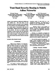
We disperse 1, 000 nodes randomly in a regular network space (see Figure 13). The zone partition is described in the figure. Each zone has averagely 40 nodes. Each node sends one message to a gateway node in each round (A round is the time for all the nodes to finish sending messages to the gateway). The zone power evaluation protocol is executed after each round. By running the max-min zPmin algorithm, we ran the algorithm for about 41000 messages before one of the hosts got saturated. By running the zone-based routing algorithm, we got about 39000 messages before the first message cannot be sent through. The performance ratio between the two algorithms in terms of the lifetime of the network is 94.5%. Without the zone structure, the number of control messages on the power of each node in every information update is 1000, and they need to be broadcasted to 1000 nodes. In zone-based algorithm, the number of control messages is just the number of the zones, 48 here, and they are broadcasted to 24 zones after the zone power evaluation. And the zone-based routing dramatically reduces the running time to find a route in our simulation. In another experiment, we disperse 1240 sensors to a square field with size 6.2 ∗ 6.2. The sensors are distributed randomly in the field. Each sensor has an initial power of 400. The power consumption formula is eij = 10 ∗ d3ij . The network
Figure 11: Maximal minimum power level path A
B
A C
B
D C
D
Figure 12: Four zones are in a square network field. The power of a zone is evaluated in four directions, left, right, up, and down. A zone is represented as a zone vertex with four direction vertices. The power labels are omitted from this figure.
5.3 6
Performance Evaluation for Zone-based Routing
Local Path Selection
For square zones k = 4 + 1 as shown in Figure 12.
105
field is divided by 5*5 squares each of which corresponds to four zones in four directions (left, right, up and down). The zone-based algorithm achieved 96% of the lifetime of the max-min zPmin algorithm.
6.
[3] Jae-Hwan Chang and Leandros Tassiulas. Energy conserving routing in wireless ad-hoc networks. In Proc. IEEE INFOCOM, Tel Aviv, Israel, Mar. 2000. [4] Benjie Chen, Kyle Jamieson, Hari Balakrishnan, and Robert Morris. Span: An energy-efficient coordination algorithm for topology maintenance in ad hoc wireless networks. In 7th Annual Int. Conf. Mobile Computing and Networking 2001, Rome, Italy, July 2001.
CONCLUSION
We have described an on-line algorithm for power-aware routing of messages in large networks dispersed over large geographical areas. In most applications that involve ad-hoc networks made out of small hand-held computers, mobile computers, robots, or smart sensors, battery level is a real issue in the duration of the network. Power management can be done at two complementary levels (1) during communication and (2) during idle time. We believe that optimizing the performance of communication algorithms for power consumption and for the lifetime of the network is a very important problem.
[5] Yu Chen and Thomas C. Henderson. S-NETS: Smart sensor networks. In Seventh International Symposium on Experiemental Robotics, Hawaii, Dec. 2000. [6] I. Chlamtac, C. Petrioli, and J. Redi. Energy-conserving access protocols for indetification networks. IEEE/ACM Transactions on Networking, 7(1):51–9, Feb. 1999. [7] A. Chockalingam and M. Zorzi. Energy efficiency of media access protocols for mobile data networks. IEEE Transactions on Communications, 46(11):1418–21, Nov. 1998. [8] B. Das, R. Sivakumar, and V. Bharghavan. Routing in ad hoc networks using a spine. In Proceedings of Sixth International Conference on Computer Communications and Networks, Sept. 1997.
It is hard to analyze the performance of online algorithms that do not rely on knowledge about the message arrival and distribution. This assumption is very important as in most real applications the message patterns are not known ahead of time. In this paper we have shown that it is impossible to design an on-line algorithm that has a constant competitive ratio to the optimal off-line algorithm, and we computed a bound on the lifetime of a network whose messages are routed according to this algorithm. These results are very encouraging.
[9] Deborah Estrin, Ramesh Govindan, John Heidemann, and Satish Kumar. Next century challenges: Scalable coordination in sensor networks. In ACM MobiCom 99, Seattle, USA, August 1999. [10] Laura Maria Feeney and Martin Nilsson. Investigating the energy consumption of a wireless network interface in an ad hoc networking environment. In INFOCOM 2001, April 2001. [11] M. Gerla, X. Hong, and G. Pei. Landmark routing for large ad hoc wireless networks. In Proceedings of IEEE GLOBECOM 2000, San Francisco, CA, Nov. 2000.
We developed an online algorithm called the max-min zPmin algorithm and showed that it had a good empirical competitive ratio to the optimal off-line algorithm that knows the message sequence. We also showed empirically that maxmin zPmin achieves over 80% of the optimal (where the optimal router knows all the messages ahead of time) for most instances and over 90% of the optimal for many problem instances. Since this algorithm requires accurate power values for all the nodes in the system at all times, we proposed a second algorithm which is hierarchical. Zone-based power-aware routing partitions the ad-hoc network into a small number of zones. Each zone can evaluate its power level with a fast protocol. These power estimates are then used as weights on the zones. A global path for each message is determined across zones. Within each zone, a local path for the message is computed so as to not decrease the power level of the zone too much.
[12] Piyush Gupta and P. R. Kumar. Critical power for asymptotic connectivity in wireless networks. Stochastic Analysis, Control, Optimization and Applications: A Volume in Honor of W.H. Fleming, pages 547–566, 1998. [13] Z. J. Haas. A new routing protocol for the reconfigurable wireless network. In Proceedings of the 1997 IEEE 6th International Conference on Universal Personal Communications, ICUPC’97, pages 562 –566, San Diego, CA, October 1997. [14] W. Rabiner Heinzelman, A. Chandrakasan, and H. Balakrishnan. Energy-efficient routing protocols for wireless microsensor networks. In Hawaii International Conference on System Sciences (HICSS ’00), Jan. 2000. [15] Chalermek Intanagonwiwat, Ramesh Govindan, and Deborah Estrin. Directed diffusion: A scalable and robust communication paradigm for sensor networks. In Proc. of the Sixth Annual International Conference on Mobile Computing and Networks (MobiCOM 2000), Boston, Massachusetts, August 2000.
Acknowledgments. This work bas been supported in part by Department of Defense contract MURI F49620-97-1-0382 and DARPA contract F30602-98-2-0107, ONR grant N0001401-1-0675, NSF CAREER award IRI-9624286, NSF award I1S-9912193, Honda corporation, and the Sloan foundation; we are grateful for this support. We thank the anonymous reviewers for their insightful and helpful comments.
7.
[16] Mario Joa-Ng and I-Tai Lu. A peer-to-peer zone-based two-level link state routing for mobile ad hoc networks. IEEE Journal on Selected Areas in Communications, 17, Aug. 1999. [17] D. B. Johnson and D. A. Maltz. Dynamic source routing in ad-hoc wireless networks. In T. Imielinski and H. Korth, editors, Mobile Computing, pages 153 –181. Kluwer Academic Publishers, 1996.
REFERENCES
[1] Jon Agre and Loren Clare. An integrated architeture for cooperative sensing networks. Computer, pages 106 – 108, May 2000.
[18] B. Karp and H.T. Kung. GPSR: Greedy Perimeter Stateless Routing for wireless networks. In Proceedings of MobiCom 2000, Aug. 2000.
[2] A.D. Amis, R. Prakash, T.H.P. Vuong, and D.T. Huynh. Max-min d-cluster formation in wireless ad hoc networks. In Proceedings IEEE INFOCOM 2000. Conference on Computer Communications, March 2000.
[19] Y. B. Ko and N. H. Vaidya. Location-aided routing (LAR) in mobile ad hoc networks. In Proceedings of ACM/IEEE MOBICOM’98, pages 66 – 75, 1998.
106
[20] P. Krishna, N.H. Vaidya, M. Chatterjee, and D.K. Pradhan. A cluster-based approach for routing in dynamic networks. Computer Communication Review, 27, April 1997. [21] Range LAN. http://www.proxim.com/products/rl2/7410.shtml. [22] A.B. McDonald and T.F. Znati. A mobility-based framework for adaptive clustering in wireless ad hoc networks. IEEE Journal on Selected Areas in Communications, 17, Aug. 1999. [23] S. Murthy and J. J. Garcia-Luna-Aceves. An efficient routing protocol for wireless networks. ACM/Baltzer Journal on Mobile Networks and Applications, MANET(1,2):183 –197, October 1996. [24] V. Park and M. S. Corson. A highly adaptive distributed algorithm for mobile wireless networks. In Proceedings of INFOCOM’97, Kobe, Japan, April 1997. [25] M.R. Pearlman and Z.J. Haas. Determining the optimal configuration for the zone routing protocol. IEEE Journal on Selected Areas in Communications, 17, Aug. 1999. [26] C. E. Perkins and P. Bhagwat. Highly dynamic destination-sequenced distance-vector routing (DSDV) for mobile computers. Computer Communication review, 24(4):234 –244, October 1994.
B
1
[27] G. J. Pottie and W. J. Kaiser. Wireless integrated newtork sensors. Communications of the ACM, 43(5):51–58, May 2000.
2
3
4
5
6
7 C
A A
[28] S. Ramanathan and M. Steenstrup. Hierarchically-organized, multihop mobile networks for multimedia support. ACM/Baltzer Mobile Networks and Applications, 3(1):101–119, June 1998.
1
2
3
4
5
******
6
[29] Volkan Rodoplu and Teresa H. Meng. Minimum energy mobile wireless networks. In Proc. of the 1998 IEEE International Conference on Communications, ICC’98, volume 3, pages 1633–1639, Atlanda, GA, June 1998.
B
*
[30] Elizabeth Royer and C-K. Toh. A review of current routing protocols for ad hoc mobile wireless networks. In IEEE Personal Communication, volume 6, pages 46 – 55, April 1999.
Figure 13: The scenario used for the zone-based experiment. The network space is a 10 ∗ 10 square with nine buildings blocking the network. Each building is of size 2∗2, and regularly placed at distance 1 from the others. The sensors are distributed randomly in the space nearby the buildings. Each sensor has an initial power of 4000. The power consumption formula is eij = 10 ∗ d3ij . We partition the network space into 24 zones, each of which is of size 1 ∗ 4 or 4 ∗ 1, depending on its layout. For each zone, there is another corresponding zone with the same nodes but with opposite direction. For example, in the upperright figure, areas 2, 3, 4, 5, 6 constitute a zone, with 2 and 6 its source and sink areas; and 6, 5, 4, 3, 2 constitute another zone with 6 and 2 its source and sink areas. We have a total of 48 zones. The right figures show the layout of the neighboring zones. In the upper figure, 3 is the sink area of the zone A, and 5 is the source area of zone C. The border area of A and B is 2, 3; and the border area of B and C is 5, 6. The lower figure shows two perpendicular zones. The source area of B is 1, 2. The border area of A and B is 1, 2, 3, 4.
[31] S. Singh, M. Woo, and C. S. Raghavendra. Power-aware routing in mobile ad-hoc networks. In Proc. of Fourth Annual ACM/IEEE International Conference on Mobile Computing and Networking, pages 181–190, Dallas, TX, Oct. 1998. [32] Adcon Telemetetry. http://www.adcon.com. [33] Ya Xu, John Heidemann, and Deborah Estrin. Adaptive energy-conserving routing for multihop ad hoc networks. Research Report 527 USC/Information Sciences Institute, October 2000.
107