Optimal Active and Reactive Power Dispatch Problem ...

Optimal Active and Reactive Power Dispatch Problem Solution using Whale Optimization Algorithm R.H.Bhesdadiya1, Siddharth A. Parmar2, Indrajit N. Trivedi3, Pradeep Jangir4, Motilal Bhoye5, Narottam Jangir6 1

Assistant Professor, Dept. of Electrical Eng., L.E. College, Morbi-363642, India, 2,4,5,6 PG Student, Dept. of Electrical Eng., L.E. College, Morbi-363642, India, 3 Associate Professor, Dept. of Electrical Eng., GEC Gandhinagar-382028, India [email protected], [email protected], [email protected], [email protected], [email protected], [email protected] R.H. Bhesdadiya1: +91-9737132353

Abstract Background/Objectives: Optimal Power Flow problem is very common and important problem for effective power system operation and planning. OPF is previously solved by many optimization techniques. Methods/Statistical analysis: To solve the optimal power flow problem, the Whale Optimization Algorithm (WOA) is employed on the IEEE-30 bus test system. It is a population-based algorithm. WOA is inspired from the bubblenet hunting strategy of humpback whales. WOA has a fast convergence rate due to the use of roulette wheel selection method. Various mathematical steps are used in the algorithm. Findings: The problems considered in the OPF problem are Fuel Cost Reduction, Active Power Loss Minimization, and Reactive Power Loss Minimization. These problems are solved by adjusting the control parameters of the system. The results obtained by WOA is compared with other techniques such as Flower Pollination Algorithm (FPA) and Particle Swarm Optimizer (PSO). Application/Improvements: Results shows that WOA gives better optimisation values for the particular case as compared with FPA, PSO and other wellknown techniques that confirm the effectiveness of the suggested algorithm. Keywords: Optimal Power Flow, Reactive Power Loss Minimization, Whale Optimization Algorithm, Active Power Loss Minimization.

1

Introduction

At the present time, The Optimal Power Flow (OPF) is a very significant problem and most focused objective for power system scheduling as well as operation1. The OPF is the elementary tool which permits the utilities to identify the economic operational and considerable secure states in the system2, 3. The prior aim of the OPF is to evaluate the optimum operational state of an electric network by minimizing a specific objective function within the limits of the operational constraints like equality constraints and inequality constraints4, 5. Hence, the Optimal power flow problem can be defined as a highly non-linear and non-convex multimodal optimisation problem6. From the past few years too many optimisation techniques were used to solve the Optimal Power Flow (OPF) problem7, 8. Some traditional methods are used to solve the proposed problem have been suffered from some limitations like converging at local optima, not suitable for binary or integer problems and also have the assumptions like the convexity, differentiability, and continuity9, 10. Hence, these techniques are not suitable for the actual OPF situation11, 12 . All these limitations are overcome by meta-heuristic optimisation methods like BHBO, TLBO, LCA, etc. In the present work, a newly introduced meta-heuristic optimisation approach named Whale Optimization Algorithm (WOA) is used to solve the problem of Optimal Power Flow. The WOA technique is a biological and sociological inspired algorithm. This technique is inspired by the bubble-net hunting strategy of the Whale13. The capabilities of WOA are finding the global solution, fast convergence rate due to the use of roulette wheel selection, can evaluate continuous and discrete optimisation problems. In the present work, the WOA is implemented for standard IEEE-30 bus test system to solve the OPF problem. There are three objective cases considered in this paper that have to be optimize using Whale Optimization Algorithm (WOA) technique are Fuel Cost Reduction, Active Power Loss Minimization and Reactive Power Loss Minimization. The result shows the optimal adjustments of control variables in accordance with their limits. The results obtained using WOA technique has been compared with Flower Pollination Algorithm (FPA) and Particle Swarm Optimisation (PSO) techniques. The results show that WOA gives better optimisation values as compared to different methods which prove the strength of the suggested method.

2

Whale Optimization Algorithm

In the meta-heuristic algorithm, a newly purposed optimization algorithm called Whale optimization algorithm (WOA), which inspired from the bubble-net hunting strategy. Algorithm describes the special hunting behavior of humpback whales, the whales follows the typical bubbles causes the creation of circular or ‘9-shaped path’ while encircling prey during hunting. Simply bubble-net feeding/hunting behavior could understand such that humpback whale went down in water approximate 10-15 meter and then after the start to produce bubbles in a spiral shape encircles prey and then follows the bubbles and moves upward the surface. Mathematic model for Whale Optimization algorithm (WOA) is given as follows13: 2.1

Encircling prey equation

Humpback whale encircles the prey (small fishes) then updates its position towards the optimum solution over the course of increasing number of iteration from start to a maximum number of iteration13. D  C . X * (t )  X (t )

(1)

X (t  1)  X * (t )  A.D

(2)

Where: A , D are coefficient vectors, t is a current iteration, X * (t ) is position vector of the optimum solution so far and X (t ) is position vector. Coefficient vectors A , D are calculated as follows: A  2a * r  a

(3)

C  2*r

(4)

Where: 𝑎⃗ is a variable linearly decrease from 2 to 0 over the course of iteration and r is a random number [0, 1]. 2.2

Bubble-net attacking method

In order to mathematical equation for bubble-net behavior of humpback whales, two methods are modeled as13: (a) Shrinking encircling mechanism

This technique is employed by decreasing linearly the value of a from 2 to 0. Random value for avector𝐴⃗in range between [-1, 1]. (b) Spiral updating position Mathematical spiral equation for position update between humpback whale and prey that was helix-shaped movement given as follows13:

X (t  1)  D '* ebt *cos(2 l )  X *(t )

(5)

Where: l is a random number [-1, 1], b is constant defines the logarithmic shape, D '  X * (t )  X (t ) expresses the distance between ith whale to the prey mean thebest solution so far. Note: We assume that there is 50-50% probability that whale either follow the shrinking encircling or logarithmic path during optimization. Mathematically we modeled as follows:  X *(t )  A.D X (t  1)   bl  D '.e .cos(2 l )  X *(t )

if if

p  0.5   p  0.5

(6)

Where: p expresses random number between [0, 1]. (c) Search for prey The vector A can be used for exploration to search for prey; vector A also takes the values greater than one or less than -1. Exploration follows two conditions D  C . X rand  X

(7)

X (t  1)  X rand  A.D

(8)

Finally follows these conditions: 

A  1 enforces

exploration to WOA algorithm to find out global optimum

avoids local optima  A  1 For updating the position of current search agent/best solution is selected. Table 1. Control Parameters of WOA

The control parameters used in the Whale Optimization Algorithm (WOA) are given in table 1. 3

Optimal Power Flow Problem Solution

As specified before, OPF is a common power flow problem that provides the optimal values of control variables by minimizing a predefined objective function with respect to the operating bounds of the system. The OPF can be mathematically calculated as3: (9) Minimize[ f (a , b)] (10) subject to s( a , b )  0 (11) And h(a , b)  0 Where, b=vector of control variables, a=vector of state variables, f (a, b) = objective function, s (a, b) = set of equality constraints, h (a, b) =set of inequality constraints. A. Variables 1. Control variables These are the variables that may be adjusted to fulfill the power flow equations. The control variables can be represented as3: (12) bT  [ PG  PG ,VG VG , QC QC , T1 TNTr ] 2

NGen

1

NGen

1

NCom

Where: PG= real power output at the generator buses not including the slack bus.VG=Voltage magnitude at generator buses.QC=Shunt VAR compensation.T= tap settings of the transformer. NGen, NTr, NCom= no. of generator units, the no. of transformers and the no. of shunt reactive power compensators, respectively. 2. State variables The variables that need to characterize the operating state of the network. The set of state variables can be represented as3: (13) aT  [ PG ,VL VL , QG QG , Sl  Sl ] 1

1

NLB

1

NGen

1

Nline

Where: PG= the real power generation at reference bus. VL= the voltage at load buses; QG= =the output of reactive power of all generators. Sl= the line flows. NLB, Nline= no. of PQ buses, and the no. of lines, respectively. B. Constraints Power system constraints may be categorized into equality constraints and inequality constraints. 1. Equality constraints

The equality constraints reveal the physical behavior of the system. These constraints are3: 1.1 Real power constraints NB (14) PGi  PDi  Vi

V j [Gij Cos( ij )  Bij Sin( ij )]  0

J i

1.2 Reactive power constraints NB

QGi  QDi  Vi V j [Gij Cos( ij )  Bij Sin( ij )]  0

(15)

J i

Where,  ij  i   j Where, NB= No. of buses, PG= the output of active power, QG= the output of reactive power, PD= real power load demand, QD= reactive power load demand, Gijand Bij= elements of the admittance matrix Yij  (Gij  jBij ) showing the conductance and susceptance among bus i and bus j, respectively. 2. Inequality constraints The inequality constraints show the bounds on electrical devices existing in the power system plus the bounds formed to surety system safety3. 2.1 Generator constraints For every generator together with the reference bus: voltage, real and reactive outputs should be constrained by the minimum and maximum bounds as follows: VGlower  VG  VGupper , i  1, ...., NGen i i i

(16)

PGlower  PGi  PGupper , i  1, ...., NGen i i

(17)

QGlower  QGi  QGupper , i  1, ...., NGen i i

(18) 2.2 Transformer constraints Transformer tap positions should be constrained inside their stated minimum and maximum bounds as follows: TGlower  TGi  TGupper , i  1, ...., NTr i i

(19)

2.3 Shunt VAR compensator constraints Shunt reactive compensators need to be constrained by their minimum and maximum bounds as follows: QClower  QGCi  QCupper , i  1, ...., NGen i i

(20) 2.4 Security constraints These comprise the bounds of a voltage at PQ buses and line flows. Each load bus Voltage should not violate from its minimum and maximum

operational bounds. Line loading over each line should not exceed to its maximum bounds. These limitations can be expressed as: VLlower  VL  VLupper , i  1, ...., NLB i i i

(21)

Sli  Slupper , i  1, ...., Nline i

(22) The inequality constraints comprise load bus voltage, the output of real power at reference bus, the output of reactive power and line flow may be encompassed as quadratic penalty functions. Penalty function can be formulated as3: 2 NLB NGen Nline (23)  lim  lim 2 max 2 Jaug  J  P  PG  PG 

1



1 

V

 (VLi VLi i 1

) Q

  S  ( Sli  Sli i 1

i 0

)

Where,  P ,  V ,  Q ,  S  penalty factors Ulim= Boundary value of the state variable U. If U is greater than the maximum bound, Ulimtakings the value of that one, if U is lesser than the minimum bound Ulimtakings the value of that bound so: U upper ; U  U upper U lim   lower ;U  U lower U

4

(24)

Application and Results

The WOA technique is implemented to resolve the OPF problem for standard IEEE 30-bus test system and for a number of cases with dissimilar objective functions. The software program is inscribed in MATLAB 2013a and applied on a 2.60 GHz i5 PC having 4 GB RAM. In the present work the WOA population size is selected to be 40. IEEE 30-bus test system With the purpose of elucidating the effectiveness of the suggested WOA technique, it is examined for the standard IEEE 30-bus system. The IEEE 30bus test system selected in this work has comprises8,9 : 6 generating units at buses 1,2,5,8,11 and 13, four tap changing transformers between buses 6-9, 6-10, 4-12, and 28-27, nine shunt reactive compensators at buses 10,12,15,17,20,21,23,24 and 29. Table 2. Limits for different control variables Table 2 shows the min-max limits for different control variables. PG is the power limit for 6 generators, VG is the voltage limits for 6 generators, Tnn is

the tap settings limits for 4 transformers, and Qc is the limits for 9 shunt compensators. In addition, the line data, bus data, generator data and the upper and lower bounds for the control variables are specified in [4], [9]. Further, fuel cost ($/h), Ploss (MW) and Qloss (MVAR) represent the total fuel cost, the active power losses and the reactive power losses, respectively. Case 1: Minimization of Generation Fuel Cost. The fuel cost reduction is the fundamental OPF objective. Hence, Y gives the total fuel cost of each generator and it is describing as: NGen (25) Y   f i ($ / h) i 1

Where, f i is the fuel cost of the i th generator. f i , may be formulated as:

(26)

fi  ui  vi PGi  wi PGi2 ($ / h) th

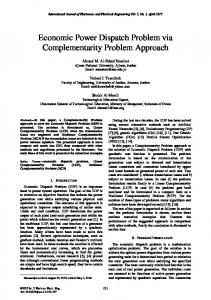
Where, ui, vi and wi are the cost coefficients of the i generator. The coefficients values are specified in [9]. Fig. 1. Fuel Cost Variations with Different Algorithms The fuel cost variations with the different algorithm can be shown in fig. 1. The optimal value of a fuel cost obtained with WOA is compared with FPA and PSO as shown in table 3. Comparison displays that WOA give better result as compared to FPA and PSO. The optimisation is done by setting the values of control variables in accordance with their limits. The control variables which are to be optimized are active power and voltage magnitudes at six generating units along with tap settings of four transformers and nine compensation devices. Table 3. Optimal Values of Fuel Costs for Different Methods Case 2: Minimization of Active Power Losses In the case 2 the Optimal Power Flow objective is to reduce the active power transmission losses, which can be represented by power balance equation as follows5: NGen NGen NGen (27) J   Pi   PGi   PDi i 1

i 1

i 1

Fig. 2. Active Power Losses Variations with Different Algorithms

Table 4. Optimal Values of PLosses for Different Methods Fig. 2 shows the tendency for reducing the total real power losses objective function using the different techniques. The active power losses obtained with different techniques are shown in table 4 which made sense that the results obtained by WOA give better values than the other methods. By means of the same settings the results achieved in case 2 with the WOA technique are compared to some other methods and it displays that the real power transmission losses are greatly reduced compared to FPA and PSO. Case 3: Minimization of Reactive Power Losses. The accessibility of reactive power is the main point for static system voltage stability margin to support the transmission of active power from the source to sinks5. Thus, the minimization of VAR losses are given by the following expression:

J

NGen

NGen

Q  Q  i 1 i 1 i

Gi

NGen

  QDi

(28)

i 1

Fig. 3. Reactive Power Losses Variations with Different Algorithms Table 5. Optimal Values of QLosses for Different Methods It is notable that the reactive power losses are not essentially positive. The variation of reactive power losses with different methods shown in fig. 3. It demonstrates that the suggested method has good convergence characteristics. The statistical values of reactive power losses obtained with different methods are shown in table 5 which displays that the results obtained by WOA are better than the other methods. It is clear from the results that the reactive power losses are greatly reduced compared to FPA and PSO. 5 Conclusion In the present work, optimal power flow problem is optimized on the IEEE 30 bus system using Whale Optimization Algorithm (WOA) technique. The results achieved by WOA method is compared with FPA and PSO techniques. The results obtained by WOA method gives better optimisation val-

ues, fast convergence and less computational time as compared to other two methods which confirms the strength of recommended algorithm. 6 Acknowledgment The authors would also like to thank Prof. Seyedali Mirjalili for his valuable support. WOA source code available at http://www.alimirjalili.com/WOA.html. 7 References 1. Duman S, Güvenç U, Sönmez Y, Yörükeren N. Optimal power flow using gravitational search algorithm. Energy Convers Manag 2012; 59:86–95. 2. H.R.E.H. Bouchekara, M.A. Abido, A.E. Chaib, R. Mehasni, Optimal power flow using the league championship algorithm: a case study of the Algerian power system, Energy Convers. Manag. 87 (2014) 58–70. 3. H.R.E.H. Bouchekara, M.A. Abido, M. Boucherma, Optimal power flow using Teaching-Learning-Based Optimisation technique, Electr. Power Syst. Res. 114(2014) 49–59. 4. A.A. Abou El Ela, M.A. Abido, Optimal power flow using differential evolution algorithm, Electr. Power Syst. Res. 80 (7) (2010) 878–885. 5. H.R.E.H. Bouchekara, Optimal power flow using black-hole-based optimisationapproach, Appl. Soft Comput. (2013). 6. S. Frank, I. Steponavice, S. Rebennack, Optimal power flow: a bibliographic survey I. Formulations and deterministic methods, Energy Syst. 3 (3) (2012)221–258. 7. M.R. AlRashidi, M.E. El-Hawary, Applications of computational intelligence techniques for solving the revived optimal power flow problem, Electr. PowerSyst. Res. 79 (4) (2009) 694–702. 8. M.A. Abido, Optimal power flow using particle swarm optimisation, Int. J. Electr.Power Energy Syst. 24 (7) (2002) 563–571. 9. K. Lee, Y. Park, J. Ortiz, A united approach to optimal real and reactive power dispatch, IEEE Trans. Power Appar. Syst. 104 (5) (1985) 1147– 1153. 10. O. Alsac, B. Stot, Optimal load flow with steady-state security, IEEE Trans. PowerApp. Syst. PAS-93 (3) (1974) 745–751. 11. T. Hariharan, K. Mohana Sundaram, “Optimal Power Flow Using Hybrid Intelligent Algorithm”,Indian Journal of Science and Technology,2015 Sep, 8(23), Doi no:10.17485/ijst/2015/v8i23/70889.

12. Meysam Rahmati, Reza Effatnejad, Amin Safari, “Comprehensive Learning Particle Swarm Optimization (CLPSO) for Multi-objective Optimal Power Flow", Indian Journal of Science and Technology, 2014 Jan, 7(3), Doi no: 10.17485/ijst/2014/v7i3/47643. 13. Seyedali Mirjalili, Andrew Lewis, “The Whale Optimization Algorithm”, ELSEVEIR-2016.

LIST OF FIGURES Fig. 1. Fuel Cost Variations with Different Algorithms Fig. 2. Active Power Losses Variations with Different Algorithms Fig. 3. Reactive Power Losses Variations with Different Algorithms

Fig.1 Fuel Cost Variations with Different Algorithms

Fig. 2 Active Power Losses Variations with Different Algorithms

Fig. 3 Reactive Power Losses Variations with Different Algorithms

LIST OF TABLES Table 1. Control Parameters of WOA Table 2. Limits for Different Control Variables Table 3. Optimal Values of Fuel Costs for Different Methods Table 4. Optimal Values of PLosses for Different Methods Table 5. Optimal Values of QLosses for Different Methods

Table 1. Control Parameters of WOA Control Parameter

Value

Population Size

40

Maximum Iteration (N)

500

Number of variable (d)

6

Random number (r)

[0,1]

Table 2. Limits for different control variables Variables

Min

Max

Variables

Min

Max

PG1

50

200

PG8

10

35

PG2

20

80

PG11

10

30

PG5

15

50

PG13

12

40

Tnn

0.9

1.1

Qc

0

5

VG

0.95

1.1

-

-

-

Table 3. Optimal Values of Fuel Costs for Different Methods Method

Fuel Cost ($/hr)

Method description

WOA

799.367


FPA

800.161

Flower Pollination Algorithm

PSO

799.704

Particle Swarm Optimizer

BHBO

799.921

Black Hole- Based Optimization5

Table 4. Optimal Values of PLosses for Different Methods Method

Plosses (MW)

Method description

WOA

2.892


FPA

3.115


PSO

3.026


BHBO

3.503


Table 5. Optimal Values of QLosses for Different Methods

WOA

Qlosses (MVAR) -25.1124


FPA

-25.056


PSO

-23.407


BHBO

-20.152


Method

Method Description