Optimal Buffer Management Using Hybrid Systems

Optimal Buffer Management Using Hybrid Systems Wei Zhang and Jianghai Hu

Abstract— This paper studies a class of dynamic buffer management problems with one buffer inserted between two interacting components. The overall system is modeled as a hybrid system and the power minimization problem is formulated as an optimal control problem. Different from many previous studies, the objective function of the proposed problem depends on the switching cost and the size of the continuous state space, making its solution much more challenging. A simplified version of the problem with some extra assumptions is solved in [1]. This paper relaxes all these assumptions and gives a complete solution to the proposed problem using some variational approach. Simulation result shows that the proposed method can save about 60% energies compared with some heuristic schemes.

I. I NTRODUCTION Dynamic buffer management (DBM) is an effective power management scheme that can reduce the power consumptions of electronic devices by inserting buffers among interacting components. The buffer insertion makes it possible to turn off underutilized components at appropriate times without affecting the services for other components, thus reducing the power consumptions. The optimal buffer size resulting in the largest power reduction is derived in [2]. The result is further extended to the case where two buffers are inserted between three streamlined components [3] [4]. A major limitation of these previous studies is that they all assume that the components to be controlled have only two power modes, “on” and “off”. However, in practice, many components can work in more than two power modes, such as variable speed processors [5] and multi-speed disks [6]. For such a component, instead of completely turning it off, we can properly design a switching strategy, namely the scheduling of different power modes of the component, to further reduce the overall power consumption. This paper studies a more general DBM problem, where the component to be controlled has multiple power modes. Since different power modes correspond to different data changing rates in the buffer, the overall system is perfectly modeled as a piecewise-constant hybrid system, or more accurately, a multi-rate automata [7]. The DBM problem is thus formulated as an optimal control problem of the underlying hybrid system. Despite the richness of the literature in optimal control of hybrid systems [8], [9], [10], [11], previous results cannot be directly applied to our problem as it has the following distinct features: (1) the discrete mode transition depends on the evolution of the continuous state; The authors are with the School of Electrical and Computer Engineering, Purdue University, West Lafayette, IN 47907, USA. Email:{zhang70, jianghai}@purdue.edu. This work was partially supported by the National Science Foundation under Grant CNS-0643805.

( r1 , p1 ) (r2 , p2 ) ry

r2

(rN , pN )

Buffer B

X Fig. 1.

Y

System Configuration

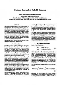
whereas most previous studies ignore such dependence; (2) the switching (mode) sequence is a decision variable that cannot be assumed fixed as in [10], [9]; (3) the switching cost ignored in most previous papers is an important part of our cost function; (4) The buffer size that determines the range of the continuous states is variable, indicating that both the optimal control and the optimal size of the state space are to be designed at the same time. Few existing results have addressed all of the above issues. A simplified version of our problem with some extra assumptions is solved in [1]. The main contribution of this paper is that we relax all the previous assumptions in [1] and give a complete analytical solution to the proposed problem, despite the challenges mentioned above. This paper is organized as follows. In Section II, we formulate the optimal control problem to be studied in this paper. In Section III, some operations on hybrid trajectories are introduced and used in deriving the optimal solutions to our problem. Simulation results are given in Section IV to illustrate the effectiveness of the proposed method. Conclusion remarks and future research directions are discussed in Section V. II. P ROBLEM F ORMULATION A. System Description Consider two interacting components X and Y as shown in Fig. 1, where X produces data for Y to consume. Suppose Y is always “on” and consumes data at a constant speed ry . On the other hand, assume that X has N different operation modes where in mode i, i = 1, 2, . . . , N , it produces data at a constant speed ri and consumes energy at the rate of pi . Without loss of generality, assume r1 < r2 < · · · < rN . Usually, a lower data processing rate corresponds to a lower power consumption; thus we require p1 < p2 < · · · < pN . Denote by I and J the sets of indices whose corresponding data rates are greater and smaller than ry , respectively, i.e.,

and

I = {i | ri > ry , i = 1, . . . , N },

J = {j | rj < ry , j = 1, . . . , N }.

Assume that both I and J are nonempty, i.e., rN > ry > r1 . A mode σ is called an ascending mode if σ ∈ I and a descending mode otherwise. To ensure smooth operation, a buffer B with capacity Q is inserted between X and Y. See Fig. 1 for the configuration of the overall system.

q(t)

q(t) Feasible Trajectory

Q

dq(t) = rσ(t) − ry , ∀t ∈ [0, tf ]. (1) dt In this paper, we study the power consumption of the whole process of transferring a certain amount of data from X to Y. It is thus required that the system must start with an empty buffer at t = 0 and end up with an empty buffer at t = tf when Y have received all the data produced by X. This yields two boundary conditions for the continuous state, namely, q(0) = 0 and q(tf ) = 0. The hybrid trajectories that satisfy these two conditions are called feasible trajectories. (See Fig. 2-(a)) We assume that there is a partition of [0, tf ], t0 = 0 ≤ t1 ≤ . . . ≤ tn = tf , for some n ≥ 0, so that σ(t) ≡ σi ∈ S is constant in each subinterval [ti−1 , ti ), i = 1, . . . , n. The sequence (σ1 , . . . , σn ) is called the switching sequence and (t0 , . . . , tn−1 ) is called the switching instants1 . A feasible trajectory is called a Λ-trajectory if it consists one ascending mode i and one descending mode j with exactly two switchings as shown in Fig 2-(b). The pair of modes {i, j} in a Λ-trajectory is called a Λ-pair. A feasible trajectory z(t) = (q(t), σ(t)) with switching instants (t0 , . . . , tn−1 ) is called a boundary-switching trajectory (BST) if q(ti ) = Q or 0 for any i = 0, . . . , n. In 1 The system is turned on at t = 0. Hence, we assume that there is always a switching at t = 0 and ignore the switching, if any, at t = tf for all trajectories.

j

i

0

q(t) Q

0

tf

(a)

B. Hybrid System Model The above problem can be modeled as a hybrid system H. The discrete state space of the hybrid system consists of N modes: S = {1, 2, . . . , N }, representing all the operation modes of X. The continuous state q(t) is defined as the amount of data stored in the buffer B, and is thus required to take values in the interval [0, Q]. The evolution of q(t) is determined by the speed difference between the two components, i.e., q(t) ˙ = ri − ry for mode i. As a physical constraint, there should be no buffer underflow or overflow. Thus we require that whenever q(t) hits the boundary of its domain, namely, q(t) = 0 or Q, the system must transit to another mode that can bring q(t) back to the inside of [0, Q]. Except for this, there are no other transition rules or guard conditions. The reset map of the system is trivial, i.e., there is no jump in q(t) at the transition instant. Given a time period [0, tf ], the behavior of the above system can be uniquely determined by the switching strategy σ : [0, tf ] → S, which determines the active mode of the system over t ∈ [0, tf ]. The overall trajectory z(t) = (q(t), σ(t)) of the hybrid system consists of the trajectories of both the continuous state q(t) and the discrete state σ(t). For a given initial state q(0), the system is governed by the following differential equation:

/ Trajectory

Q

q(t)

Boundary Switching Trajectory i3

{ i1 , j1}

0

Pure Trajectory

Q

j3

{ i2 , j2 }

{ i, j}

{ i1 , j1}

tf

(c) Fig. 2.

tf

(b)

0

{ i, j}

{ i, j}

(d)

tf

Illustration of different hybrid trajectories

other words, a BST only switches at the boundary of the range of q(t). Denote by Ω the class of all BSTs. Every BST can be decomposed into a series of Λ-trajectories with the same buffer size. Denote by np the number of distinct Λ-pairs in a BST. For example, for the BST in Fig 2-(c), we have np = 3. A BST is called pure if np = 1 and is called mixed otherwise. In other words, a pure trajectory must be a BST and is obtained by repeating a Λ-trajectory for a certain number of times. (See Fig. 2-(d)). The power consumption of a given hybrid trajectory z(t) = (q(t), σ(t)) consists of three parts: the running power, namely the power consumed by component X2 , the switching power and the buffer power. Since σ(t) ∈ S determines the active power mode of X, pσ(t) is the instantaneous power of X at time R t t. Thus the average running power over [0, tf ] is t1f 0 f pσ(t) dt. Assume that switching among different modes costs the same amount of energy ks 3 . Then the average switching power over [0, tf ] is nks /tf , where n is the number of switchings in the trajectory z. The buffer power is proportional to the buffer size Q and denoted by pb Q, where pb is a positive constant. Therefore, the total average power of the system during [0, tf ] can be written as Z nks 1 tf ¯ + pb Q. (2) pσ(t) dt + P (z; Q, tf ) = tf 0 tf Similarly, the total energy associated with z(t) during [0, tf ] is Z tf pσ(t) dt + nks + pb Q · tf . E(z; Q, tf ) = 0

The three terms on the right hand side of the above equation represent the running energy, the switching energy, and the buffer energy, respectively. C. Problem Statements

The main purpose of this paper is to find a feasible trajectory that can finish a given task with the least energy 2 The power of Y is ignored in this paper since it is a constant independent of the switching strategy. 3 There may exist other switching penalties, such as the switching delay penalty. To simplify discussion, we assume all the switching penalties are transformed to an equivalent energy cost and incorporated into ks .

consumption. This problem can be formulated as the following optimal control problem of the hybrid system H. Problem 1: Find a feasible trajectory z(t) over [0, tf ] and a proper buffer size Q that  Z tf 1 ¯ pσ(t) dt + nks + pb Q minimize P (z; Q, tf ) = tf 0 dq(t) subject to = rσ(t) − ry , with q(0) = 0, (3) dt q(tf ) = 0, max q(t) ≤ Q, and min q(t) ≥ 0. (4) t∈[0,tf ]

t∈[0,tf ]

A simplified version of Problem 1 is solved in [1] under two additional assumptions: (a) tf approaches infinity, and (b) z is periodic. In next section, we relax both of these assumptions and give a complete analytical solution to Problem 1.

III. O PTIMAL S OLUTIONS A. Operations on Hybrid Trajectories We first introduce some useful operations on hybrid trajectories: (i) Denote by Ca,b [z] the cropping operation that only keeps the part of z within the time interval [a, b], i.e., Ca,b [z](t) = z(t + a), for t ∈ [0, b − a]. (ii) Let z1 = (q1 , σ1 ) and z2 = (q2 , σ2 ) be two hybrid trajectories with length tf 1 and tf 2 , respectively. Denote by J [z1 , z2 ] the joining operation, which obtains a new trajectory by appending z2 to the end of z1 . To preserve the continuity of the continuous state, the trajectories to be joined must have consistent boundary conditions, i.e., q1 (tf 1 ) = q2 (0). In particular, suppose z1 satisfies that q1 (0) = q1 (tf 1 ). Denote by Jm [z1 ] a special joining operation that repeats z1 for m times. (iii) The scaling operation of z with parameter c is defined as: Sc [z] = (cq(t/c), σ(t/c)). The scaling operation does not change the switching sequence; however, the switching instants, the optimal buffer size and the length of z becomes c times the original values. B. Necessary Conditions To avoid the unnecessary power consumption by the unused buffer space, Q should be chosen as small as possible so that the buffer is full at least once during [0, tf ]. Thus the following lemma follows immediately. Lemma 1 (Tightness condition): If z(t) = (q(t), σ(t)) is an optimal solution to Problem 1 (OS1), we must have min q(t) = 0,

t∈[0,tf ]

and

max q(t) = Q.

t∈[0,tf ]

The following lemma is the key result of this paper and can greatly simplify the derivation of the optimal solution to Problem 1 (OS1). Lemma 2: If z is an OS1, then z ∈ Ω. Proof: Let z(t) be an OS1 with switching sequence (σ1 , . . . , σn ) and switching instants (t0 , . . . , tn−1 ). Suppose that z(t) has a switching at some interior point of [0, Q], i.e., 0 < q(ti ) < Q for some i. Divide z(t) into three parts through the cropping operation as shown in Fig. 3-(a) and define them as three new trajectories. z (1) (t) = C0,ti−1 [z](t), and

z (2) (t) = Cti−1 ,ti+1 [z](t),

z (3) (t) = Cti+1 ,tf [z](t).

(5)

Assume that z (2) (t) = (q (2) (t), σ (2) (t)), q (2) (0) = q1 and q (2) (τi ) = q2 , where τi = ti − ti−1 . Thus z (2) has an interior switching from σi to σi+1 at instant τi . Perturb this switching instant to a neiboring value h and define a (2) (2) (2) perturbed trajectory zh = (qh (t), σh (t)) as

(2) σh (t) (2)

=



σi σi+1

t≤h (2) , h < t ≤ th

dqh (t) (2) =rσ(2) (t) − ry , for t ∈ [0, th ], h dt h(ry − rσi ) + q2 − q1 (2) and th =h + . rσi+1 − ry

(6)

(2)

As illustrated in Fig. 3-(b), zh switches from σi to σi+1 (2) at time h instead of τi and ends at th where the new (2) continuous state evolves to q2 . An important property of qh (2) is that it has the same initial and final value as q (t), i.e., (2) (2) (2) (2) qh (0) = q1 and qh (th ) = q2 . Thus we can join zh with (1) (3) (1) (2) (3) z and z to obtain zh , J [z , zh , z ]. It is obvious that the length of zh is (2)

thf = ti−1 + th + (tf − ti+1 ).

(7)

Since q(ti ) ∈ (0, Q), there exist ǫ1 > 0 and ǫ2 > 0 such that ∀h ∈ Dh , [τi − ǫ1 , τi + ǫ2 ], zh (t) stays inside [0, Q] all the time. Thus ∀h ∈ Dh , zh is a properly defined trajectory for the original buffer size Q and the average power of zh is 1 P¯ (zh ; Q, thf ) = h E1 + E3 + nks + pσi h tf  (2) + pσi+1 (th − h) + pb Q,

(8)

where E1 and E3 are the running energy of z (1) and z (3) , respectively. The above perturbation on ti results in a zh with length thf 6= tf . To make zh feasible for Problem 1, define zˆh = Sch [zh ] as shown in Fig. 3-(c), where ch = tf /thf . According to the properties of the scaling operation, the buffer size of zˆh becomes cQ and the length of zˆh is changed back to tf . Therefore, zˆh is a feasible trajectory for Problem 1. The average power of zˆh with buffer ch Q can be easily computed as: 1 P¯ (ˆ zh ; Q, tf ) = h E1 + E3 + 2ks + pσi · h tf  nks (1 − ch ) (2) . + pσi+1 (th − h) + pb ch Q + ch thf

q (t )

z Q

q (t )

q (t ) (1)

q1 q2

z Vi

(2)

z

ti 1 ti

z Q

(1)

E3

z

t

tf

h

ti1

ti

C. Optimal Pure Trajectory In this section we derive analytical solutions to Problem 1 with an additional constraint np = 1, i.e., we only consider pure trajectories as candidate solutions. We call the solution to Problem 1 under this additional constraint the optimal pure trajectory (OPT). q (t )

z 1 (t )

ti1 t

h f

t

tf

ch h

E3

chti 1 chti

c t

(2) h h

tf

t

(c) zˆh with length tf

The simplest pure trajectory is the Λ-trajectory. Let z1 (t) be a Λ-trajectory as shown in Fig. 4-(a) with length tf and Λ-pair {i, j}. Since tf is fixed, its optimal buffer size is given by: tf =

Qij Qij tf + ⇒ Qij , , ri − ry ry − rj αij

(10)

where αij is defined as the ratio of the time horizon Tij to the optimal buffer size Qij for the given Λ-pair {i, j}. Denote by βij the running power of z1 , i.e.,   Qij pi Qij pj 1 + βij = Tij ri − ry ry − rj   1 pi pj = . (11) + αij ri − ry ry − rj

Note that both αij and βij are constants only depending on the given Λ-pair. The general pure trajectory with the Λpair {i, j} and 2m switchings can be obtained from z1 as zm = Jm [S1/m [z1 ]]. As shown in Fig. 4-(b), zm has an optimal buffer size Qij /m and its average power is

pb t f 2mks + . (12) P¯ij (m) = βij + tf mαij Taking the derivative of P¯ij (m) with respect to m and setting it to zero, we obtain the optimal value of m as r pb m ˆ ij = tf . (13) 2ks αij Note that the parameter m must be an integer, and the function P¯ij (m) is convex in m. Therefore, if m ˆ ij is not an integer, the optimal feasible value of mij , m∗ij , is whichever of the two closest integers to m ˆ ij that results in the smallest value of P¯ij (m) as defined in (12). Hence, m∗ij =

arg min

P¯ij (m).

(14)

m∈{⌊m ˆ ij ⌋,⌈m ˆ ij ⌉}

{σ + , σ − } = arg min P¯ij (m∗ij ).

j

(15)

{i∈I,j∈J}

Q

ij

m tf (a) Fig. 4.

Vi

The minimal achievable power for any pure trajectory with the Λ-pair {i, j} is P¯ij (m∗ij ). Then the best Λ-pair {σ + , σ − } can be obtained as

z m (t )

Q

ij

0

t

(2) h

[z h ]

V i 1

E1

E3

Taking the derivative of P¯ (ˆ zh ; Q, tf ) with respect to h, we have   dP¯ (ˆ zh ; Q, tf ) ry − rσi 1 pσi + pσi+1 =  2 dh rσi+1 − ry thf     ry − rσi q2 − q1 − 1+ · tf −(ti+1 −ti−1 )+ rσi+1 − ry rσi+1 − ry   q2 − q1 · E1 + E3 + ks + pσi+1 rσi+1 − ry   ry − rσi nks − pb Qtf 1 − + . rσi+1 − ry (thf )2 (9) Note that the h-related terms in the numerator have been ¯ ;Q,Th ) cancelled out. From (9) it is clear that the sign of dP (zhdh ¯ does not depend on h, which indicates that P (ˆ zh ; Q, thf ) is monotone with respect to h in Dh = [τi − ǫ1 , τi + ǫ2 ]. Thus either zτi −ǫ1 or zτi −ǫ2 consumes a less power than z. Therefore, we conclude that q(ti ) = 0 or Q for all i = 1, . . . , n, i.e., the OS1 must be a BST. Lemma 2 allows us to consider only the BSTs in deriving the OS1s. Recall that the variable np is used to describe the purity of a BST. In the rest of this section, we will first solve a simple case of Problem 1 where only pure BSTs with np = 1 are considered as candicate solutions. Then we will prove that the optimal solution in this simple case is also an OS1 for an arbitrary np .

i

ch q1 ch q2

฀ ch

h

˜ = h + ti−1 , t˜(2) = t(2) + ti−1 . Illustration of the proof of Lemma 2, where h h h

Fig. 3.

Q

zˆ

chQ

(b) Perturbed zh (t)

(a) z(t) with interior switching

q (t )

z

(3)

Vi E1

ti 1

(2) h

V i 1

q1 q2

V i1

E1

(3)

2

1

0

……

tf m

Obtaining zm from z1

(b)

m

tf

Denote by Σf the set of all minimizers of (15). Thus if {i, j} ∈ Σf , then an OPT can be obtained by repeating the Λ-trajectory with the pair {i, j} for m∗ij times. Thus the following theorem follows immediately.

q (t )

z

Q

m1 , m2

Proof: To simplify the notations, let c = pb t2f , a1 = βi1 ,j1 αi1 ,j1 tf , and a2 = βi2 ,j2 αi2 ,j2 tf . Relax m1 , m2 to nonnegative real numbers x1 and x2 . Then

(t ) i2

j1

i1

1

2

……

m1

1

Fig. 5.

E(x1 , x2 ) = 2ks (x1 + x2 ) +

…… m 2

0 m1D i1 j1 Q

j2

m2D i2 j2 Q

tf

An example of zm1 ,m2 (t)

Theorem 1: Let zm (t) be a pure trajectory as shown in Fig. 4-(b) with 2m switchings and Λ-pair {i, j}. If {i, j} ∈ Σf and m = m∗i,j , then zm is an OPT with optimal buffer size Qij /m∗ij .

Note that all the constants a1 , a2 , c, αi1 ,j1 , and αi2 ,j2 are positive. To prove the lemma, it suffices to show that there exists a point on the x1 or x2 axis that minimizes E(x1 , x2 ) in the first quadrant. To find the minimizers of E(x1 , x2 ) in the first quadrant, we can first minimize it along each ray in the first quadrant, and then find the ray that gives the best minimum value. Towards this purpose, define x2 = λx1 , where λ ∈ [0, ∞]. Then (a1 + a2 λ)x1 + c E(x1 , λx1 ) =2ks (1 + λ)x1 + (αi1 ,j1 + αi2 ,j2 λ)x1 s 2ks (1 + λ)c (a1 + a2 λ) ≥2 + αi1 ,j1 + αi2 ,j2 λ (αi1 ,j1 + αi2 ,j2 λ) ,E(x∗1 , λx∗1 ).

D. General Optimal Solution In last subsection, we derive analytically the optimal pure trajectories with np = 1. A natural question is that whether the power can be further reduced if we relax the constraint on np . To answer this question, we start with a simple case where candidate trajectories are allowed to contain at most two distinct Λ-pairs,4 i.e., np ≤ 2. Let zm1 ,m2 be a BST consisting of m1 copies of Λ-pair {i1 , j1 } and m2 copies of Λ-pair {i2 , j2 }. Without loss of generality, assume that all the same pairs are grouped together as shown in Fig 5. In other words, the switching sequence of zm1 ,m2 is assumed to take the following form (σ1 , . . . , σ2(m1 +m2 ) ) = (i1 , j1 , . . . , i1 , j1 i2 , j2 , . . . , i2 , j2 ). | {z }| {z } m1 pairs

m2 pairs

For a given pair of m1 and m2 , the optimal buffer size of zm1 ,m2 is uniquely determined by Q=

a1 x1 + a2 x2 + c . αi1 ,j1 x1 + αi2 ,j2 x2

tf , αi1 ,j1 m1 + αi2 ,j2 m2

where αi,j is the ratio of the time duration to the optimal buffer size for the Λ-pair {i, j} as defined in (10). Let βi,j be the running power of the pair {i, j} as defined in (11). Then the total energy consumed by zm1 ,m2 is computed as E(m1 , m2 ) = 2(m1 + m2 )ks + pb t2f + βi1 ,j1 αi1 ,j1 m1 tf + βi2 ,j2 αi2 ,j2 m2 tf . αi1 ,j1 m1 + αi2 ,j2 m2 Lemma 3: For any {i1 , j1 } and {i2 , j2 }, there exists a pair of nonnegative integers (m∗1 , m∗2 ) with either m∗1 = 0 or m∗2 = 0 such that E(m∗1 , m∗2 ) ≤ E(m1 , m2 ) for any other pair of nonnegative integers (m1 , m2 ). 4 Two different Λ-pairs may consist of three or four different modes. For example, {σ1 , σ2 } and {σ1 , σ3 } are also called two different Λ-pairs although they have one mode in common.

Thus E(x∗1 , λx∗1 ) is the minimum value achieved on the ray x2 = λx1 . To prove the lemma, it suffices to show that either λ = 0 or λ = ∞ minimizes E(x∗1 , λx∗1 ). After some computations, E(x∗1 , λx∗1 ) reduces to s 1 a2 ∗ ∗ + d1 y + , f (y), E(x1 , λx1 ) =d3 d2 y + αi2 ,j2 αi2 ,j2 where √ d1 = a1 αi2 ,j2 − a2 αi1 ,j1 , d2 = αi2 ,j2 − αi1 ,j1 and d3 = 2 2ks c are all constants and y=

αi22 ,j2 λ

1 . + αi1 ,j1 αi2 ,j2

Note that except d1 and d2 , all the other constants are positive. As λ increases from 0 to ∞, y decreases from 1 αi1 ,j1 αi2 ,j2 to 0. Hence, it suffices to show that either 0 or 1 1 αi1 ,j1 αi2 ,j2 is a minimizer of f (y) in [0, αi1 ,j1 αi2 ,j2 ]. Note that the second-order derivative of f (y) is d22 d3 d2 f (y) = − ≤ 0. 2 dy 4(d2 y + 1/αi2 ,j2 )3/2 Thus f (y) is a concave function of y in [0, αi ,j 1αi ,j ]. Since 1 1 2 2 the minimizer of a concave function over a bounded set must be on the boundary of the set, we conclude that either 0 or 1 1 αi1 ,j1 αi2 ,j2 is a minimizer of f (y) in [0, αi1 ,j1 αi2 ,j2 ]. According to Lemma 3, for any given two Λ-pairs, we can always use one of them to construct a pure trajectory that performs equally well or better than all the other mixed trajectories involving these two Λ-pairs. Therefore, the following corollary follows immediately. Corollary 1: The OPT is an optimal solution to Problem 1 under an additional constraint np ≤ 2. The question now becomes that whether we can save more energy by further relaxing the constraint on np . It turns out to be not the case. In fact, the OPT is an optimal solution to Problem 1 for an arbitrary np . This can be proved by

IV. S IMULATION

TABLE I P OWER MODES OF I NTEL X SCALE P ROCESSOR 1 150 0.45 0.08

2 400 1.2 0.17

3 600 1.8 0.4

4 800 2.4 0.9

5 1000 3 1.6

Let X be an Intel Xscale processor [5] with five available power modes as defined in Table I. Suppose that Y is a video card that fetches data from X at a constant speed 8 Mbps (1MB/s). The power per megabyte for buffer B is 6.258 × 10−4 W/MB [4]. A typical value of the switching energy is 0.1mJ in a microprocessor [13]. Since the switching cost ks in our model may also include other switching penalties, such as the switching delay penalty, we will test our method for ks ranging from 0.1mJ to 100mJ. A heuristic strategy is implemented where X is switched to the highest speed until the buffer is full and then switched to the lowest speed until the buffer is empty. This method is referred to as Scheme2 while Scheme1 refers to the optimal strategy as defined in Theorem 1. Scheme2 is tested for four heuristically selected buffer sizes 0.1MB, 0.3MB, 1MB and 8MB. The power consumptions of Scheme2 in these cases are compared with Scheme1 in Fig. 6. It is clear that our optimal strategy always performs the best for each ks and can save more than 60% of power consumptions compared with the other strategy. V. C ONCLUSIONS A dynamic power manage problem is formulated as an optimal control problem of a hybrid system. By exploiting of the particular structure of our system model, the optimal solutions are derived analytically based on some variational approach. Simulation result based on real data shows that the proposed method can save 60% energies compared with a heuristic scheme. Future research will focus on the following

Scheme1 Scheme2(Q=0.1MB) Scheme2(Q=0.3MB) Scheme2(Q=1MB) Scheme2(Q=8MB)

0.8

0.6

0.4

0.2

0

Our theoretical results can be applied in many real-world applications, such as the power management problem of a multiple-speed disk [6] and the dynamic voltage scheduling (DVS) problem of a variable speed processor [5]. In this section, we use a DVS example to illustrate the effectiveness of our results.

mode i fi (MHz) ri (MB/s) pi (Watt)

1

Normalized Power

induction. The following lemma is the key of the induction procedure. Lemma 4: For any BST z with length tf and np = l + 1, there exists another BST zˆ with length tf and np ≤ l that consumes equal or less power than z. Remark 1: Note that Lemma 4 is not a trivial application of Lemma 3. Its proof is much longer and is thus omitted. Interested reader can refer to [12] for a complete proof. According to Lemma 4, any BST corresponds to a pure trajectory with np = 1, thus the following theorem follows immediately. Theorem 2: The OPT defined in Theorem 1 is an OS1 for an arbitrary np .

0

0.01

0.02

0.03

0.04

0.05

0.06

0.07

0.08

0.09

0.1

k s(J)

Fig. 6. Power consumptions of various methods under different ks . For each ks , all the powers are normalized w.r.t. the largest one.

two aspects: one is to extend our analysis to the case with more than one buffers inserted among multiple streamlined components. The other one is to study the case where the data rates of components are varying or even random instead of constant. R EFERENCES [1] W. Zhang, J. Hu, and Y. H. Lu. Optimal power modes scheduling using hybrid systems. to appear in the Proceedings of the American Control Conference, 2007. [2] L. Cai and Y.-H. Lu. Energy management using buffer memory for streaming data. IEEE Transactions on Computer-Aided Design of Integrated Circuits and Systems, 24(2):141–152, 2005. [3] J. Hu and Y.-H. Lu. Buffer management for power reduction using hybrid control. In Proceedings of the IEEE Conference on Decision and Control, pages 6997–7002, Seville, Spain, 2005. [4] J. Ridenour, J. Hu, N. Pettis, and Y.-H. Lu. Low-power buffer management for streaming data. IEEE Transactions on Circuits and Systems for Video Technology, 17(2):143–157, 2007. [5] R. Xu, C. Xi, R. Melhem, and D. Moss. Practical pace for embedded systems. In EMSOFT ’04: Proceedings of the 4th ACM international conference on Embedded software, pages 54–63. ACM Press, 2004. [6] S. Gurumurthi, A. Sivasubramaniam, M. Kandemir, and H. Franke. Drpm: Dynamic speed control for power management in server class disks. In Proceedings of the International Symposium on Computer Architecture (ISCA), pages 169–179, June 2003. [7] R. Alur, T. Henzinger, G. Lafferriere, and G. J. Pappas. Discrete abstractions of hybrid systems. Proceedings of the IEEE, 88(2):971– 984, 2000. [8] S. Hedlund and A. Rantzer. Optimal control of hybrid system. In Proceedings of the IEEE Conference on Decision and Control, volume 4, pages 3972–3977, Phoenix, AZ, December 1999. [9] M. Egerstedt, Y. Wardi, and F. Delmotte. Optimal control of switching times in switched dynamical systems. IEEE Transactions on Automatic Control, 51(1):110–115, 2006. [10] X. Xu and P.J. Antsaklis. Optimal control of switched systems based on parameterization of the switching instants. IEEE Transactions on Automatic Control, 49(1):2–16, 2004. [11] S. C. Bengea and R. A. DeCarlo. Optimal control of switching systems. Automatica, 41(1):11–27, 2005. [12] W. Zhang and J. Hu. Optimal buffer management using hybrid systems. to be submitted for journal publication. [13] T. D. Burd and R. W. Brodersen. Design issues for dynamic voltage scaling. In Proceedings of the international symposium on Low power electronics and design, pages 9–14. ACM Press, 2000.