Optimal Feature Selection for Context-Aware Recommendation using ...

Optimal Feature Selection for Context-Aware Recommendation using Differential Relaxation Yong Zheng, Robin Burke, Bamshad Mobasher Center for Web Intelligence School of Computing, DePaul University Chicago, Illinois, USA {yzheng8,rburke,mobasher}@cs.depaul.edu

ABSTRACT Research in context-aware recommender systems (CARS) usually requires the identification of the influential contextual variables in advance. In collaborative recommendation, there is a substantial trade-off between applying context very strictly and achieving good coverage and accuracy. Our prior work showed that this tradeoff can be managed by applying the contexts differentially in different components of the recommendation algorithm. In this paper, we extend our previous model and show that our differential context relaxation (DCR) model can also be used to identify demographic and item features that are linked to the contexts. We also demonstrate the application of binary particle swarm optimization as a scalable optimization technique for deriving the optimal relaxation.

Categories and Subject Descriptors H.3.3 [Information Systems]: Information Search and Retrieval

General Terms Algorithms, Modeling, Optimization

Keywords Context-aware recommender systems, collaborative filtering, differential context relaxation, particle swarm optimization

1.

INTRODUCTION

Context-aware recommender systems (CARS) extends the focus of recommender systems research beyond users and items to the contexts in which items are experienced by users, attempting to model the interactions that are often influential in making good recommendations. For example, Alice may prefer causal restaurants with spicy Thai food when dining with friends, but would rather choose a quiet but upscale Italian place when entertaining work colleagues. Clearly, the occasion (work vs. personal life) and the companions (friends vs. co-workers) play a key factor in what a system should recommend. The recognition of the importance of such contextual factors is a starting point for much CARS research.

—————————————————————————————– CARS-2012, September 9, 2012, Dublin, Ireland. Copyright is held by the author/owner(s).

What we see in this example, however, is that these contextual factors (occasion, companions) are linked to specific features associated with the restaurant itself: the type of food, the atmosphere, perhaps the price. To the extent that such linkages are shared among many users, we call these context-linked features. When contextual information is limited, we may be able to observe context-linked features more readily, and so discovering influential context-linked features is an important goal for CARS research. In our previous research [16], we developed a context-aware collaborative recommendation approach based on differential context relaxation (DCR). The differential aspect of the algorithm is that we segment the recommendation algorithm into different components and apply different aspects of the context to each part. Each component of the algorithm operates on the same collaborative user-item-rating data, but only those parts that match its particular context. The context relaxation part of the algorithm arises because we treat the context as a set of constraints controlling what data is available to a given component. Finding the optimum set of contextual features then becomes a matter of finding a relaxation of these contextual constraints so that a balance between accuracy and coverage is achieved. In this paper, we show that context-linked features are also good candidates for our relaxation technique. Previously, we used a data set with only a handful of contextual variables so it was possible to do an exhaustive search of all possible relaxations in order to find the optimum. In this work, we show that binary particle swarm optimization (BPSO) [10] can be applied to find optimal relaxations with a larger set of context and context-linked variables.

2.

RELATED WORK

CARS researchers have sought different means of discovering influential contextual variables. Baltrunas et al [2] conducted a survey asking subjects to evaluate the importance of contextual factors to acquire contextual relevances. Others [15, 7] applied feature selection or reduction techniques to extract influential contexts from a set of candidate variables. However, each of these techniques has its drawbacks: the technique in [2] requires a lot of user effort; the feature reduction techniques are not reliable unless the data set is dense across contexts – items have been rated multiple times in different contexts. Comparing with explicit contextual approaches above, there are also approaches incorporating latent factors: previously we applied labeled-LDA to infer contexts based on review mining[6]. A. Karatzoglou et al [8] introduced multiverse recommendation based on a N-dimensional tensor factorization model, and L. Baltrunas et al [3] present a novel context-aware recommender based on matrix factorizations. In this paper, we mainly focus on the existing explicit contextual features we already know, and we will incorporate

latent factor models in the future. Rather than seeking to define a set of contextual variables to be applied to the algorithm as a whole, our previous work [16] sought to decompose collaborative recommendation into components and apply different aspects of the context to each. We think of the context as a constraint governing what data each component considers and seek the strongest constraint consistent with low error and acceptable coverage. Note that this concept of constraining the data used by different parts of the recommendation algorithm is quite different from constraint-based recommendation, in which constraints are applied to the recommended items themselves [5].

3.

METHODOLOGY

We take as our starting point the well-known Resnick’s algorithm for collaborative recommendation: P (ru,i − r¯u ) × sim(a, u) u∈N P (1) Pa,i = r¯a + sim(a, u) u∈N

where a is a user, i is an item, and N is a neighborhood of other users u similar to a. The algorithm calculates Pa,i , which is the predicted rating that user a is expected to assign to item i. The algorithm can be understood as operating over the rating data in three different ways. r¯a averages over all of the ratings supplied by user a to establish an overall baseline for the target user. The formation of the neighborhood N requires selecting all users for their similarity to a. And, finally, r¯u is computed for each user u to establish their baseline rating to be subtracted from their individual rating of item i. Contextual effects may enter into the algorithm in various ways. Perhaps a user has a different baseline rating in different contexts. For example, Alice, our hypothetical diner, may have relatively low expectations for her casual Thai restaurants and give a lot of high scores but give out relatively few five star ratings for her workoriented experiences. Perhaps good collaborative peer groups are context-specific – recommendations from expense-account-wielding business types might be good for her work dinners but not for anything else. To account for this kind of variance, we start with the target context C, which is the context for which the recommendation is sought. Our prediction now is for target user a, item i, and context C: how will the user respond to this item in this context? For example, how will Alice like a fancy regional American restaurant in the “work” context with Betsy, her boss and Carl, an out-of-town client? It is unlikely that other users will have dined with exactly the same individuals before, which is why we want to think of controlling recommendation based on constraints derived from C as opposed to C itself. For example, we may want to generalize Alice’s dining occasion as a small work event, which would exclude peer experiences where the meal was a large banquet. From the target context, we derive three sets of contextual constraints: C1 , C2 , C3 and apply them to these components separately, yielding the following context-sensitive formulation: P (ru,i,C2 − r¯u,C2 ) × sim(a, u) Pa,i,C = r¯a,C3 +

u∈NC1

P

sim(a, u)

(2)

u∈NC1

This version of the equation replaces N with NC1 , meaning that we only consider neighbors who have rated item i in a context matching C1 . Instead of averaging over all ratings when normalizing peer ratings, we select only those ratings in contexts matching

C2 , and we do a similar thing for the target user by matching against C3 . In our previous work, we were able to show significant improvement in accuracy for hotel recommendation in a travel data set (http://www.tripadvisor.com/) with the following constraints: C1 (neighbor filtering) using “state of origin”, C2 (peer baseline) using “trip type” (e.g. business, family, etc), and no constraints on target user baseline, C3 = {}, where trip type is known as a typical influential context [6], and we found the state of origin was another one. For more details, see [16]. What is significant here is that each of the three components of the algorithm worked best with their input data filtered in different context-related ways. We derived this result by evaluating all possible sets of constraints on all of the data and finding the optimum combination.

3.1

Optimization of Constraint Search

We model the relaxation as a process of binary selection – we represent C1 , C2 and C3 as binary vectors where a bit value of one denotes that we filter the data using that feature. In extending this work to other data sets and adding context-linked features, it became clear that an optimization approach based on exhaustive search was not scalable. To some extent, regularities in the data and dependencies between the variables can shrink the combinatorial space. For example, in our travel data set, origin city was fixed for each user, meaning that whether we restricted it or ignored it, the computation was the same when computing a user’s baseline. So, that variable only became relevant for neighborhood calculation. There were other similar simplifications for the other components, and we imagine that this would be true of most recommendation domains. Even with such simplifications, we require a more scalable optimization technique than exhaustive search. Furthermore, the optimization space is highly non-linear and standard approaches such as gradient descent cannot be used. However, we have had success with the particle swarm optimization technique.

3.2

Particle Swarm Optimization

Particle swarm optimization (PSO) [9] is a kind of swarm intelligence which was originally introduced by Eberhart and Kennedy in 1995. It is a population-based optimization approach inspired by social behaviors in swarming and flocking creatures like bees, birds or fish. It was introduced to the domain of information retrieval [4] and recommender system [1, 14] recently as a way for feature selection and feature weighting. Binary particle swarm optimization (BPSO) is a discrete binary version of the technique introduced in 1997, which is used to fit our binary selections for contexts and feature relaxation in this paper. The basic idea behind PSO is that optimization is produced by a number of particles at different points in an optimization space. Each particle searches independently for the optimum, guided by the local value and communication with the other particles. In our case, we use RMSE as the value to be minimized and the position in the space corresponds to a set of constraints. Each particle i records its personal best performance (iBest) and corresponding best position (Pibest ). The algorithm also keeps track of the global best performance (gBest) and corresponding position (Pgbest ). In each iteration of the algorithm, each particle moves through the optimization space as a function of its velocity. The velocity is a function of an inertia term and represented by functions of iBest and gBest. The inertia is gradually decreased over time so that the particles will be more influenced by the previously-located minima. The update formulas for Vij (the velocity of j th bit in particle i)

and the global inertia w are as follows: j Vij,t = wt × Vij,t−1 + α1 ϕ1 × (Pibest − Xij,t−1 ) j +α2 ϕ2 × (Pgbest − Xij,t−1 )

(3)

where ϕ1 and ϕ2 are positive random numbers drawn from a uniform distribution between 0.0 and 1.0, α1 and α2 are constant learning factors (set as 2.0 by empirical suggestions [13]) which control the weight given to the local and the global minima, respectively. Xij,t is the particle’s position (the value of j th bit in particle i) at the iteration t. Usually velocity is restricted within range [−Vmax , Vmax ]. It cannot be too fast or too slow – a small velocity will result in minor changes on the positions, where large velocity will drive the particle to move too much in the space. Vmax is suggested to be the maximum value of each bit in the position vector, where in our case it is 1 because the value switches between 0 and 1. Further experiments show that 2.0 is a better configuration. The inertia at a given iteration t is calculated by: wt = wend +

(Tmax − t) × (wstart − wend ) Tmax

(4)

where Tmax denotes the maximum number of iterations. The designer specifies a starting and ending weight with wstart > wend . A large inertia weight value facilitates a global search while a small value facilitates a local search. The linear decreasing value means that the algorithm begins with the particles being more influenced by their current direction and ends with them being more influenced by their neighbors. We followed the empirical parameter configuration: wstart = 0.9 and wend = 0.4, which is suggested in PSO research [13]. The velocity is used to update the value (position) Xij of each bit in the binary vector. Basically, the higher the velocity, the greater probability of switching to 1.   1, if (randt < S(Vij,t )) Xij,t = (5) 0, otherwise 1 where S(Vij,t ) = 1+exp(−V , which is a sigmoidal function ij,t ) squashes the range of velocity to a range of [0,1]. randt is a uniform random number in the range [0,1]. In our application, we use from 1 to 5 particles initialized with a random velocity and random bit vectors representing the possible constraints. For each iteration, every particle runs our algorithm across the training set, compares the RMSE it acquires in current iteration with the best so far (pBest and gBest), and updates them as well as the corresponding positions. Then the new position for next iteration is generated based on the equations above. The ability of the particles to communicate within the swarm reduces the total number of iterations required to reach an optimum.

3.2.1

Improved BPSO

Whether each bit value in the binary vector for each particle is 1 or 0 actually depends on the value of velocity – if the velocity is larger, it is more like it is to switch to 1. Thus the weakness of classical BPSO is that it only considers the possibility of change to 1, and does not take the possibility of change to 0 into account. Mojtaba et al [11] improved BPSO by taking the possibility of change to 0 into the consideration. Consider the best position visited so far for a particle is Pibest and the global best position for the particle is Pgbest . Assume the j th bit of ith best particle is 1. So to guide the bit j th of ith particle to its best position, the velocity of change to one for that particle should be increased and the velocity

of change to zero should be decreased. Then the improvement can be described as follows: j If Pibest = 1 Then d1ij,1 = α1 r1 and d0ij,1 = −α1 r1 j If Pibest = 0 Then d0ij,1 = α1 r1 and d1ij,1 = −α1 r1 j If Pgbest = 1 Then d1ij,2 = α2 r2 and d0ij,2 = −α2 r2 j If Pgbest = 0 Then d0ij,2 = α2 r2 and d1ij,2 = −α2 r2 where d1ij and d0ij are two temporary values and r1 and r2 are two random variable in range of (0,1). α1 and α2 are the same learning factors. With this in mind, we define two separate velocities, one in the “1” direction V 1 and one in “0” direction V 0 .

Vij1

Vij1 = wVij1 + d1ij,1 + d1ij,2

(6)

Vij0 = wVij0 + d0ij,1 + d0ij,2

(7)

Vij0

We choose or as the velocity, depending on the current position of the particle for that bit.  1  Vij , if (Xij,t−1 = 0) Vij,t = (8) Vij0 , if (Xij,t−1 = 1) Finally the bit value can be updated as follows:   X ij,t−1 , if (randt < S(Vij,t )) Xij,t = Xij,t−1 , otherwise

(9)

where X ij,t−1 denotes the 2’s complement of Xij,t−1 ; that is, if Xij,t−1 = 0, then X ij,t−1 =1; otherwise, X ij,t−1 =0. Our experiments show this improved version can find optimum more efficiently than classical BPSO.

4.

EXPERIMENTAL SETUP

For this paper, we use a rating data set in the area of food, the "AIST context-aware food preference dataset" which was used and distributed by the author Hideki Asoh [12]. The data set was generated using a survey of 212 users asking them to rate items on a menu. There were two different conditions in the survey. In one condition, “real hunger”, users were asked to rate the items based on their current degree of hunger. In the “virtual hunger” situation, they were asked to imagine a degree of hunger different from the current state and asked what their preferences would be in that state. Asoh and his colleagues collected 6,360 ratings for 20 food menus, and also included demographic and item features in the data. Each user supplied 30 ratings. For our exploration of contextual recommendation, we use 6 variables. The key contextual variable is degree of hunger (real or virtual), but we also wanted to explore context-linked features including gender and various item features related to the food that were available in the data. Food genre indicates the food is Chinese, Japanese or Western food; food stuff denotes the food category is vegetable, pork, beef, or fish, and the food style contains values that represent the style of food preparation. The data set is split into five folds where each user has at least one rating in each fold. For each fold, we used DCR to come up with the optimal combinations of context and context-linked features. We compare this technique to collaborative filtering without contexts and with contextual pre-filtering which is the similar to the Equation 2 where C2 and C3 are null are we only constrain the neighbor selection. In order to determine the value of context-linked features, we created two additional test conditions looking at the contextual feature alone (degree of hunger) and using the contextual feature together with context-linked features (demographic and item features discussed above).

5.

EXPERIMENTAL RESULTS

Recall that we want to discover influential contexts and contextlinked features, and our method for doing so is to find the optimal set of constraints and see what features are contained therein. Our results show that on this data set appropriate relaxation of contexts and features can help improve predictive performance, and incorporating context-linked features outperforms using contexts only.

5.1

Predictive Performance

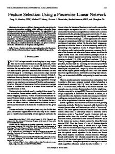
The experimental results are shown in Figure 1 and Table 1. We use CO to denote contextual features (degree of hunger) and CL to denote the other demographic and item features that we suspect may be context-linked. These are the results achieved by exhaustive search; the optimization results are as below. 1.215

100.0%

1.200

99.7% 99.4%

1.185

99.1%

1.170

98.8%

RMSE (Bar)

1.155 98.5% 1.140

Coverage (Line)

98.2% 1.125

97.9%

1.110

97.6%

1.095

97.3% 97.0%

1.080

Standard CF Pre!filtering Pre!filtering Pre!filtering (CL) (CO) (CO+CL)

RMSE

DCR (CL)

DCR (CO) DCR (CO+CL)

Coverage

Figure 1: Comparison of Predictive Performance As the figure shows, the contextual pre-filtering and our DCR model can make improvements comparing with the standard CF without incorporating contexts, and the DCR model achieved the best RMSE among these algorithms. Besides, DCR shows better accuracy improvement when context-linked features are added, but it does not work for contextual pre-filtering. We believe the effects shown by adding context-linked features are domain-specific. And those features should be applied to appropriate components in the model, where DCR using CL only and DCR using CO and CL together provide significant improvements in terms of RMSE. But pre-filtering restricts the application of context-linked features for neighborhood filtering only. – it may not provide accuracy improvements; instead, more restrict constraints may bring lower coverage as shown in the figure above. We also examined coverage. When the dataset is sparse, introducing contextual constraints can greatly limit coverage, an effect that we found in our previous research. With this dataset, there was little cost in coverage – the best coverage is 99.7% by standard CF model, while the best DCR model shows a 99.3% coverage. Notice that when contexts are introduced into the 1st algorithm component (neighbor filtering), the coverage may depend on which variables are selected as the relaxed ones for this component, as well as the density of contextual information in the data set. From Figure 1 and Table 1, we can see the coverage of pre-filtering using both context and context-linked features is the lowest, because real hunger and gender together as more strict constraints are selected and applied in this component.

5.2

Analysis of the Optimal Constraints

Table 1 shows how the different conditions yield different optimal constraints. For pre-filtering and DCR using contextual features only, the real hunger is influential. When context-linked features are added, real hunger is still influential, but it is applied to different components in the DCR model. Context-linked features can provide accuracy improvements but it has to be applied to appropriate components – the best DCR model is using all of the algorithm components, the pre-filtering part of the algorithm retains only “gender” and the hunger-related features are applied elsewhere. Context-linked features - gender, food genre, food stuff, food style are selected and applied in the optimal model. The position of contextual constraints in the optimal relaxation is also telling. “Gender” turns out to be the best feature for C1 , indicating that same-sex peer neighborhoods work best in this domain. Also, we see that a fully restricted constraint – all contexts and food features appear in C2 , which is where we choose the ratings to be used in constructing the peer user’s baseline rating. It confirms the assumption by CARS – users’ preferences differ from contexts to contexts, thus neighbor’s exactly matched contextual ratings contribute significantly to predict user’s rating on the same item under the same contexts. The optimal model took real hunger as the only constraint in 3rd component, which implies the users’ average rating under the same real hunger situation works the best as the representative of this component.

5.3

Optimization Performance

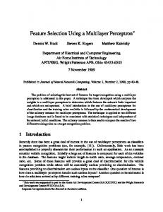
It is clear that differential context relaxation is useful both for improving algorithm performance and discovering crucial features. However, exhaustive search is not a practical or scalable way to realize this goal, although it is possible in this data set. We used this data set as an opportunity to experiment with BPSO as an alternative method of finding the optimal context relaxation. We examined particle counts from 1 to 5, using a maximum of 100 iterations. A local minimum occurred in classical BPSO – it converged an RMSE (1.116) not quite as good as the global minimum found by exhaustive search (1.114). The improved BPSO algorithm does find the global minimum RMSE and the same set of relaxations as the exhaustive search. Figure 2 shows the learning curve of the improved version, where N -BPSO denotes we use number of N particles in the swarm. Improved BPSO finds the 1 BPSO

RMSE

In order to assess the effectiveness of our particle swarm technique, we performed exhaustive search of the constraint space (8,192 iterations) and compared this result with that found by the optimization technique.

3 BPSO

5 BPSO

1.210 1.200 1.190 1.180 1.170 1.160 1.150 1.140 1.130 1.120 1.110 1.100 1

6 11 16 21 26 31 36 41 46 51 56 61 66 71 76 81 86 91 96 Number of Iterations

Figure 2: Improved BPSO optimal solutions on average around the 18th iteration using one particle, and 12th iteration using five particles. 18 iterations with 1 particles corresponds to 18 evaluations over the training set, a more than 455× reduction in computational cost. Increasing the number of particles expands the power of social contributions by other particles, and can reduce the number of iterations, but also increases

Dataset: Food Menu Standard CF Pre-filtering (CL) Pre-filtering (CO) Pre-filtering (CO+CL) DCR (CL) DCR (CO) DCR (CO+CL)

RMSE 1.203 1.202 1.198 1.204 1.163 1.119

Coverage 99.7% 99.3% 99.6% 98.3% 99.7% 99.6%

1.114

99.3%

Table 1: Optimal Relaxations Optimal Relaxation N/A C1 = {gender} C1 = {real hunger} C1 = {real hunger, gender} C1 = {}; C2 = {food genre, food stuff, food style}; C3 = {food genre, food stuff, food style} C1 = {real hunger}; C2 = {}; C3 = {real hunger} C1 = {gender}; C2 = {real hunger, virtual hunger, food genre, food stuff, food style}; C3 = {real hunger}

the amount of computation per iteration. The selection of the number of particles and the number of iterations depends on the specific cost and computational complexity of the algorithm.

6.

CONCLUSIONS

Differential context relaxation is a technique for context-aware recommendation that decomposes the recommendation algorithm into components and filters the data used in each component. The context is considered a set of constraints, which may be relaxed to achieve the best recommendation performance. In this work, we examine an optimization technique – binary particle swarm optimization – to efficiently locate the highest performing set of contextual constraints. We show that BPSO can find the global optimum constraint set with a fraction of the iterations required by exhaustive search. We also show that both contextual features and context-linked features can be useful in our context relaxation model. Furthermore, our algorithm highlights the different roles that contextual features play, producing some interesting results, such as the fact that same-sex neighbor populations work best in our food data set. Future research will be focused on two parts: 1) exploring the possibility for real-valued (as opposed to binary) definition of differential context relaxation and 2) applying the same technique to additional algorithms beyond user-based collaborative filtering. 3) combine with the latent factor models, such as matrix factorization in order to alleviate the sparsity problem of contextual ratings and examine our differential model in another way.

7.

[6]

REFERENCES

[1] A. Abdelwahab, H. Sekiya, I. Matsuba, Y. Horiuchi, and S. Kuroiwa. Feature optimization approach for improving the collaborative filtering performance using particle swarm optimization. Journal of Computational Information Systems, 8(1):435–450, 2012. [2] L. Baltrunas, B. Ludwig, S. Peer, and F. Ricci. Context relevance assessment and exploitation in mobile recommender systems. Personal and Ubiquitous Computing, pages 1–20, 2011. [3] L. Baltrunas, B. Ludwig, and F. Ricci. Matrix factorization techniques for context aware recommendation. In Proceedings of the fifth ACM conference on Recommender systems, pages 301–304. ACM, 2011. [4] H. Drias. Web information retrieval using particle swarm optimization based approaches. In Web Intelligence and Intelligent Agent Technology (WI-IAT), 2011 IEEE/WIC/ACM International Conference on, volume 1, pages 36–39. IEEE, 2011. [5] A. Felfernig and R. Burke. Constraint-based recommender systems: technologies and research issues. In Proceedings of

[7]

[8]

[9]

[10]

[11]

[12]

[13]

[14]

[15]

[16]

the 10th international conference on Electronic commerce, ICEC ’08, pages 3:1–3:10, New York, USA, 2008. ACM. N. Hariri, B. Mobasher, R. Burke, and Y. Zheng. Context-aware recommendation based on review mining. In Proceedings of the 9th Workshop on Intelligent Techniques for Web Personalization and Recommender Systems (ITWP 2011), page 30, 2011. Z. Huang, X. Lu, and H. Duan. Context-aware recommendation using rough set model and collaborative filtering. Artificial Intelligence Review, pages 1–15, 2011. A. Karatzoglou, X. Amatriain, L. Baltrunas, and N. Oliver. Multiverse recommendation: n-dimensional tensor factorization for context-aware collaborative filtering. In Proceedings of the fourth ACM conference on Recommender systems, pages 79–86. ACM, 2010. J. Kennedy and R. Eberhart. Particle swarm optimization. In Neural Networks, 1995. Proceedings., IEEE International Conference on, volume 4, pages 1942–1948. IEEE, 1995. J. Kennedy and R. Eberhart. A discrete binary version of the particle swarm algorithm. In Systems, Man, and Cybernetics, 1997. Computational Cybernetics and Simulation., 1997 IEEE International Conference on, volume 5, pages 4104–4108. IEEE, 1997. M. Khanesar, M. Teshnehlab, and M. Shoorehdeli. A novel binary particle swarm optimization. In Control & Automation, 2007. MED’07. Mediterranean Conference on, pages 1–6. Ieee, 2007. C. Ono, Y. Takishima, Y. Motomura, and H. Asoh. Context-aware preference model based on a study of difference between real and supposed situation data. User Modeling, Adaptation, and Personalization, pages 102–113, 2009. Y. Shi and R. Eberhart. Empirical study of particle swarm optimization. In Evolutionary Computation, 1999. CEC 99. Proceedings of the 1999 Congress on, volume 3. IEEE, 1999. S. Ujjin and P. Bentley. Particle swarm optimization recommender system. In IEEE Swarm Intelligence Symposium, pages 124–131. IEEE, 2003. B. Vargas-Govea, G. González-Serna, and R. Ponce-Medellín. Effects of relevant contextual features in the performance of a restaurant recommender system. In ACM RecSys’ 11, the 3rd Workshop on Context-Aware Recommender Systems (CARS-2011), 2011. Y. Zheng, R. Burke, and B. Mobasher. Differential context relaxation for context-aware travel recommendation. In 13th International Conference on Electronic Commerce and Web Technologies (EC-WEB 2012), volume 123 of Lecture Notes in Business Information Processing, pages 88–99. Springer Berlin Heidelberg, 2012.