OPTIMAL GOSSIP ALGORITHM FOR DISTRIBUTED CONSENSUS SVM TRAINING IN WIRELESS SENSOR NETWORKS K. Flouri1 , B. Beferull-Lozano2 , and P. Tsakalides1 1
Department of Computer Science University of Crete and Institute of Computer Science (FORTH-ICS) 71110 Heraklion, Crete, Greece {flouri,tsakalid}@ics.forth.gr ABSTRACT In this paper, we consider the distributed training of a SVM using measurements collected by the nodes of a Wireless Sensor Network in order to achieve global consensus with the minimum possible inter-node communications for data exchange. We derive a novel mathematical characterization for the optimal selection of partial information that neighboring sensors should exchange in order to achieve consensus in the network. We provide a selection function which ranks the training vectors in order of importance in the learning process. The amount of information exchange can vary, based on an appropriately chosen threshold value of this selection function, providing a desired trade-off between classification accuracy and power consumption. Through simulation experiments, we show that the proposed algorithm uses significantly less measurements to achieve a consensus that coincides with the optimal hyperplane obtained using a centralized SVM-based classifier that uses the entire sensor data at a fusion center. Index Terms— Convex optimization, SVMs, consensus, gossip algorithms, wireless sensor networks 1. INTRODUCTION With the advent of wireless sensor networks, there has been a growing interest towards decentralized detection, estimation and classification algorithms for use in monitoring, surveillance, location sensing, and distributed learning applications. Moreover, the development of visual sensor networking technology will require efficient distributed processing for automated event detection and classification. Most of the problems that occur in WSN applications, can be expressed as This work was supported by GSRT under program ΠENE∆, Code 03E∆69, the Marie Curie TOK-DEV “ASPIRE” grant (MTKD-CT-2005029791) within the 6th European Community Framework Program, and the spanish MEC Grants TEC2006 10218 “SOFIWORKS” and CONSOLIDERINGENIO 2010 CSD2008-00010 “COMONSENS”
2
Escuela T´ecnica Superior de Ingenier´ıa (ETSI) Instituto de Rob´otica Universidad de Valencia (UV) 46071, Valencia, Spain
[email protected] distributed optimization problems. In [1], an incremental optimization algorithm is presented for robust estimation of a cost function of interest, applied to energy-based source localization, clustering, and density estimation. More recent studies in distributed optimization have mainly focused on estimating simple functions of the data, analyzing issues such as convergence criteria and convergence rate [2, 3]. Moreover in [4], power consumption has been taken into account for the algorithmic design. An important class of distributed algorithms employ the so-called gossip techniques. They seem well suited in the context of a WSN, since neighboring sensors can exchange data to diffuse information in the network. For this reason, gossip techniques are robust to changes in the topology of the network in case of node failures. They are based on successive refinement of local estimates maintained at individual sensors. Gossip-based approaches rely on communication with one-hop neighbors only, to develop iterative algorithms that eventually converge to the desired estimate. After some iterations, all sensors reach consensus to the optimal solution. The notion of consensus averaging for the estimation of deterministic unknown parameters using linear data models was introduced in [5] whereby each sensor updates its local estimate by appropriately weighting the estimates of its neighbors. A more elaborate approach entailing distributed computation of the sample average estimator with the aid of dual decomposition techniques was studied in [6]. For distributed estimation of a Gaussian random parameter in a scalar linear model, [7] applied the Jacobi iteration. More recently, a consensus-based distributed expectation-maximization algorithm was proposed in [9] for density estimation and classification. Finally, in [10], a distributed strategy is developed that enables a subset of the nodes to calculate any given function of the node values. Support Vector Machines constitute a modern classification tool, that has been successfully applied to a number of applications ranging from face recognition and text categorization to engine knock detection, bioinformatics, and database
marketing [11, 12, 13]. Training involves optimization of a convex cost function meaning that there are no false local minima to complicate the learning process. SVMs are the most well-known of a class of algorithms that use the idea of kernel substitution and which are broadly referred to as kernel methods. SVMs can also construct linear classification functions with good theoretical and practical generalization properties even in very high-dimensional attribute spaces. The major advantage of linear classifiers is their simplicity and low complexity. In general, pattern classification algorithms assume that all the features are available centrally during the construction of the classifier and its subsequent use. But in many practical situations, data are recorded in different geographical locations by sensors, each observing features of local interest and having a partial view of the data. We first proposed in [14] a distributed algorithm for training a SVM in the context of a WSN, exchanging only partial information among sensors (the so-called support vectors). Through analytical studies and simulation experiments, we showed that the distributed algorithm exhibits similar performance to the traditional centralized SVM training method, while being much more efficient in terms of energy cost. Independently of our work, Vandenberghe et al. proposed a distributed parallel SVM training mechanism based on the same idea of exchanging support vectors among multiple servers in a strongly connected network [15]. In [16], Navia-Vazquez provided distributed semiparametric SVM, which aims at further reducing the total information passed between nodes. Finally in [17], an SVM scheme is applied to distributed image classification in a sensor network. In this paper we provide a mathematical characterization for the sparse representation of the most important measurements that neighboring nodes should exchange in order to reach an agreement near the optimal SVM classifier. We introduce a selection function which ranks each training vector in order of importance. Therefore, the amount of information exchange can vary allowing for a a desired trade-off between classification accuracy and power consumption. The main contributions of this paper are: • The mathematical characterization of the required partial information that neighboring sensor nodes should exchange in order to achieve consensus in the network, while minimizing the number of transmissions. • The design of the corresponding gossip algorithm achieving global consensus with minimal inter-node network communication. This paper is structured as follows. In Section 2, we describe the problem of centralized SVM training as a convex optimization problem. Section 3 formulates the distributed consensus SVM problem and Section 4 describes the theoretical foundation (selection function) of our method and the corresponding gossip algorithm. Experimental results are provided in Section 5, while conclusions are drawn in Section 6.
2. CENTRALIZED SVM TRAINING AS A CONVEX OPTIMIZATION PROBLEM In this Section, we provide a brief description of training a SVM classifier, assuming that all the computation is performed in a centralized manner at a certain fusion center. This convex optimization problem can be described mathematically using several equivalent formulations, each of them having a concrete geometrical interpretation. Consider a binary classification task with data vectors xi , i = 1, . . . , n from class {+1} and yj , j = 1, . . . , m from class {-1}. Assume that these data sets are linearly separable1 . Intuitively, the plane that best separates the data sets, is the one further from both classes. With this choice of hyperplane, small changes in the data will not yield misclassification errors. Thus, intuitively, one is interested in constructing a hyperplane that maximizes the minimum distance from the plane to each set. A plane supports a class if all points in that class are on one side of that plane. For the points in class {+1} and class {-1}, the goal is to find a vector w and an offset b such that w · xi + b ≥ 1 and w · yj + b ≤ −1, respectively. This problem turns out to be a convex optimization problem [18], which can be formulated as follows: kwk2 min 2 (1) subject to wT · xi + b ≥ 1, i = 1, . . . , n wT · yj + b ≤ −1, j = 1, . . . , m. Using optimization duality theory [18], it is possible to obtain an equivalent alternative formulation given by: Pm Pn min k i=1 θi xi − j=1 γj yj k2 θ,γ Pm Pn (2) subject to j=1 γj = 1, i=1 θi = 1, θi ≥ 0, γj ≥ 0. where θ = [θ1 , . . . , θn ], γ = [γ1 , . . . , γm ]. In the framework of optimization theory, convex optimization problems (1) and (2) are said to be dual of each other. Observing (2), one can easily notice that it can be interpreted as the problem of finding the minimum distance between two convex hulls: the convex hull that contains the data xi of one class and the convex hull that contains the data yj of the other class. The optimal discriminant (classifier) is defined by vector w∗ and offset b∗ as follows: n∗ m∗ X X ∗ ∗ w = θi xi − γj∗ yj , (3) i=1
j=1
b∗ = 1 − w∗T xi , or b∗ = 1 − w∗T yj .
(4)
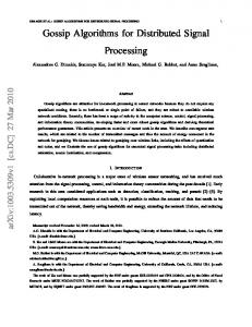
Notice that the resulting separating hyperplane is expressed by means of a linear combination of the so-called support vectors, i.e., those xi 0 s, yj 0 s corresponding to non-zero θi∗ , γj∗ , respectively. This is illustrated in Figure 1, where the support vectors 9, 12 construct the discriminant w∗ . 1 The generalization of the results of this paper to the case of non-linear separation and to more than two classes is part of our current research and will be presented elsewhere.
w*
1
7
2 6 3
4
Fig. 1. Optimal hyperplane is orthogonal to the shortest segment connecting the convex hulls of the two classes and it can be constructed using only the two support vectors (vectors 9 and 12). 3. DISTRIBUTED CONSENSUS SVM TRAINING Consider a simple case where the network is composed of two sensors. Each sensor collects n measurements from class {1} and m measurements from class {-1}. We define these (1) (1) (1) (1) two sets as following, S1 := {x1 , . . . , xn , y1 , . . . , ym } (2) (2) (2) (2) and S2 := {x1 , . . . , xn , y1 , . . . , ym }. We want to train a SVM and therefore classify all the measurements in the network. In the ideal case with no power constraints in the network, each sensor sends their data to a fusion center where the SVM is trained on the whole data set S := S1 ∪ S2 . The hyperplane is constructed from the support vectors (cf. Eq. (3)). Let SVS be the set that contains the support vectors obtained when the training is performed with all the data (centralized case). Clearly, SV S ⊂ S. Moreover, notice that if s ∈ SV S , then s ∈ S1 or s ∈ S2 . A distributed training strategy can reduce significantly the power consumption in a WSN [14]. Since the data of each node can be compressed to their corresponding estimated hyperplane and thus to the associated support vectors, one could expect that the support vectors are the sufficient data to send to the neighboring sensors in order to construct the optimal hyperplane. However, it turns out is that in general, a support vector in the centralized case, may not be a support vector in the subproblems. This is illustrated clearly in Figure 2. Training locally the SVM for the data collected by sensor 1 (S1), the support vectors that construct the discriminant are vectors 2 and 6. Similarly, for the data collected by sensor 2 (S2), the support vectors are vectors 3 and 7. In the centralized case, as illustrated in Figure 2, the support vectors are 1, 4, 5 and 7. Notice that vectors 1, 4, and 5 are not support vectors in the subproblems of sensor 1 or sensor 2. Hence, the straightforward idea that sensors exchange only their corresponding support vectors and update their local solutions cannot guarantee convergence to the optimal SVM classifier, as claimed in [15].
5
Fig. 2. Example of a case where the global SVM solution makes use of a vector which is not a support-vector in neither of the two subproblems associated to each of the sensors. Vectors 1, 4 and 5, become support vectors of the global SVM solution. The question at this point is what kind of information should neighboring sensors exchange in order to get the best possible classification accuracy while keeping the power consumption low. In [19], we proposed, independently of [15] two distributed algorithms: a) the MSG-SVM, where the minimum amount of data corresponding to the support vectors of each node, is selected for diffusion; and b) the SSG-SVM, where sufficient data corresponding to the vectors defining the convex hull of each class is diffused to achieve optimality, that is, same performance as a global centralized algorithm. MSG-SVM provides a sub-optimal solution, while SSG-SVM achieves optimality but with an additional power cost. In Section 4, we provide a mathematical characterization of the importance of a vector sample as to be selected for exchange with other neighboring sensors. This allows us to judiciously choose the partial information that neighboring sensors should communicate in order to achieve consensus in the network, while limiting the communication cost. We provide a selection function which ranks the training vectors in order of importance in the learning process of the SVM classifier. As we will see next, the amount of information exchange can vary, based on an appropriately chosen threshold value that is applied to this selection function, providing a desired tradeoff between classification accuracy and power consumption. 4. ADAPTIVE SELECTIVE GOSSIP ALGORITHM 4.1. The Selection Function Consider the optimization problem as defined by (2). Since this problem is convex, optimality is achieved when the Karush Kuhn Tucker (KKT) conditions are satisfied. In other words, if (θ ∗ , γ ∗ ) are the optimal values, then for i = 1, . . . , n, and j = 1, . . . , m: −θi∗ ≤ 0, −γj∗ ≤ 0, Pn Pm ∗ ∗ ∗ ∗ i=1 θi = j=1 γj = 1, λi ≥ 0, µj ≥ 0
(complementary slackness), −λ∗i θi∗ = 0, −µ∗j γj∗ = 0, ∇L(θ ∗ , γ ∗ , λ∗ , µ∗ , ν1∗ , ν2∗ ) = 0, where (λ∗ , µ∗ , ν1∗ , ν2∗ ) are the optimal Lagrange multipliers (dual variables). The Lagrangian of (2) can be expressed as follows: L(θ, γ, λ, µ, ν1 , ν2 ) = n m n ³X ´ X X k θi xi − γj yj k2 +ν1 θi − 1 i=1
+ν2
j=1
m ³X
´ γj − 1 −
j=1
n X
i=1 m X
λi θi −
i=1
µj γj .
j=1
The partial derivatives with respect to θi , γj , are X ∂L = 2θi k xi k2 +2 θk < xi , xk > ∂θi k6=i X −2 γl < xi , yl > −λi + ν1 , l X ∂L = 2γj k yj k2 +2 γl < yl , yj > ∂γj l6=j X −2 θi < xi , yj > −µj + ν2 . i
Substituting the optimal values θ = θ ∗ and γ = γ ∗ , the KKT conditions must hold,X which results in : X 2θi∗ k xi k2 +2 θk∗ < xi , xk > −2 γl∗ < xi , yl >
4.2. Geometrical Interpretation of the Selection Function In Section 2, we emphasized that in SVMs, the resulting separating hyperplane is expressed by means of a linear combination of the support vectors, (cf. (3)). The support vectors are the closest points to the hyperplane among all the measurements of each class. The expression for the hyperplane is w∗ T xi + b∗ = 0. The distance of a measurement xi of class {1} from the hyperplane is given by: d2 (xi , w∗ ) =
k w∗ T xi + b∗ k2 . k w∗ k2
(5)
For a measurement xi of class {1}, since the hyperplane is determined by (3), it follows that: 1 (6) xTi w∗ = F (xi ). 2 Therefore, from (5) and (6), it can be concluded that: (F (xi )/2 + b∗ )2 . (7) k w∗ k2 This is a very interesting observation, because for a fixed b∗ ∈ R, the function (F (xi )/2 + b∗ )2 is monotonically increasing since by definition, w∗ T xi + b∗ > 1. Similarly, it can be d2 (xi , w∗ ) =
(F (y )/2−b∗ )2
j shown that yTj w∗ = − 12 F (yj ), d2 (yj , w∗ ) = . kw∗ k2 ∗ 2 Again, the function (F (yj )/2−b ) is monotonically increask6=i l ∗ ∗ ing for a fixed b∗ ∈ R, since w∗ T yj + b∗ < −1. Therefore, = λi − ν1 , as the value of F (xi ) increases, so does d2 (xi , w∗ ). Since X X ∗ 2 ∗ ∗ d(xi , w∗ ) > 1 by definition, (cf. (1)), then as d2 (xi , w∗ ) in2γj k yj k +2 γl < yl , yj > −2 θi < xi , yj > creases, the distance increases as well. Similarly for class i l6=j {-1}, as the value of F (yj ) increases, so does the distance of = µ∗j − ν2∗ . yj from the hyperplane. In other words, by calculating the selection function for From complementary slackness, at optimality λ∗i θi∗ = 0, each measurement, we have information about the distance of and µ∗j γj∗ = 0. Therefore λ∗i = 0 when θi∗ 6= 0, i = 1, . . . , n each measurement to the hyperplane. Notice that the support and µ∗j = 0 when γj∗ 6= 0, j = 1, . . . , m. In conclusion, vectors have the smallest value of the selection function for if xi , yj are not support vectors, then the above expressions each class, since they are the closest points to the hyperplane. do not change. On the other hand, if xi , yj are support vecIn this way, all the training vectors can be ranked in order tors and hence λi = µj = 0, then they can be expressed as of importance in the learning process. Given a desired tradefollows: off between classification accuracy and power consumption, X X 2θi∗ k xi k2 +2 θk∗ < xi , xk > −2 γl∗ < xi , yl > = −ν1∗ , the amount of information exchange can vary, based on userdefined threshold values F1 and F2 of the respective selection k6=i l X X functions. The greater the values of the thresholds, the more 2γj∗ k yj k2 +2 γl∗ < yl , yj > −2 θi∗ < xi , yj >= −ν2∗ . data will be exchanged to neighboring sensors.
l6=j
i
We now define a selection function F (xi ), F (yj ) for each 4.3. The ASG-SVM Algorithm vector xi , yj , respectively as follows: X X We now introduce the Adaptive Selective Gossip (ASGθk∗ < xi , xk > −2 γl∗ < xi , yl >,SVM) algorithm, where the vectors of the set Selected Setk (t) F (xi ) = 2θi∗ k xi k2 +2 k6=i l selected by each sensor at time t, are communicated to all X X (k) ∗ 2 ∗ ∗ F (yj ) = 2γj k yj k +2 γl < yl , yj > −2 θi < xi , yj >its. one-hop neighbors. Given threshold values F1 and (k) F2 , the set of vectors to be transmitted and exchanged i l6=j by a certain sensor at the initial time step t = 0, is deterThis selection function can be calculated locally at each sen(k) sor for all its measurements. mined as: Selected Setk (0) = {xi : F (xi ) < F1 , i =
50
centralized ASG−SVM 50% MSG−SVM SSG−SVM ASG−SVM 30%
0.2
40 35
Number of vectors
Percentage of misclassified data
ASG−SVM 50% MSG−SVM SSG−SVM ASG−SVM 30%
45
0.25
0.15
0.1
30 25 20 15 10
0.05 5
0 1
2
3
4
5
0 1
2
3
4
5
Iterations
Iterations
(a)
(b)
Fig. 3. a) Performance, at a given particular sensor, of the training algorithms. MSG-SVM is a suboptimal solution but finally reaches the optimal plane. ASG-SVM and SSG-SVM give an optimal estimate of the discriminant after 3 iterations. The ideal case where sensors have access to the entire data is depicted by the straight line. b) MSG-SVM gives a sub-optimal solution using less measurements than the other algorithms. Even though both ASG-SVM and SSG-SVM give the optimal solution, ASG-SVM uses less data than SSG-SVM at each iteration. (k)
1, . . . , n} ∪ {yj : F (yj ) < F2 , j = 1, . . . , m}. The vectors of the set Selected Setk (t) selected by each sensor at time t, are communicated to all its one-hop neighbors. Therefore, for each node k, at time t + 1, we update its estimate wk∗ (t + 1) by using all the information available at that moment, namely, the previously estimated set of the support vectors SVk (t) at node k, as well as the union of the sets Selected SetNk (t) that have been previously generated by the neighboring nodes using the selection functions. A description of the algorithm for each sensor k is the following: INPUT • Data set Sk contains the measurements collected by the k-th sensor. (k)
• Set the thresholds F1
(k)
and F2 .
PROCEDURE 1. Initialize time slot t=0, and the set Sk := Sk (0). 2. Train the SVM on the current data set Sk , and obtain optimal hyperplane w∗k (t) ( ≡ set of support vectors SVk (0)). 3. Calculate F (xi ) and F (yj ) for the measurements xi of class {1} and yj of class {−1}, respectively. 4. Determine Selected Setk (t) 5. Transmit Selected Setk (t) to neighboring sensors Nk . To save power, transmit only those vectors that were not transmitted to neighboring sensors in previous time slots.
6. Update Sk (t + 1) = {SVk (t) ∪ Selected SetNk (t)}. 7. Increment t, and return to Step 2, if Selected Setk (t) 6= ∅. OUTPUT • Hyperplane w∗k (t) that classifies the data at sensor k. 5. RESULTS We consider a sensor network composed of k = 10 nodes distributed in a grid topology, where each sensor collects 10 {xi }10 i=1 , {yj }j=1 sample vectors from two classes, at each time slot. In our experiments, we generated a data set of two different classes each, using Gaussian distributions with two different means. We simulated 100 Monte Carlo runs in order to test the performance of three selective gossip algorithms, namely MSG-SVM, SSG-SVM poposed in [19] and the ASG-SVM introduced in this work. We note that in MSG-SVM only the support vectors are exchanged among sensors. In that sense, MSG-SVM is similar to DPSVM in [15]. On the other hand, in SSG-SVM all vectors determining the convex hull are passed to the neighboring sensors. Figure 3a illustrates the average classification error rates (%) for two randomly chosen sensors, as a function of the iteration steps. In this scenario, the 30% and the 50% of the measurements of each sensor is chosen to be exchanged among neighboring sensor. In the centralized case, the two classes are linearly separable and therefore the misclassification error rate is zero. MSGSVM exhibits a slightly lower performance than the other algorithms, which is expected since less information (only
the support vectors) is communicated. On the other hand, SSG-SVM and ASG-SVM achieve the same performance when the 50% of the measurements are exchanged after. This illustrates that although each algorithm transmits different data, both of them transmit a sufficient amount of data in order to achieve optimality. Finally, ASG-SVM, when the %30 of the measurements are exchanged, exhibits better performance than MSG-SVM algorithm (%25 of the measurements are exchanged). Figure 3b illustrates the number of measurements that a particular sensor transmits to its neighbors at each iteration. MSG-SVM gives a sub-optimal solution but uses less measurements than ASG-SVM and SSG-SVM, thus less power. Even though SSG-SVM and ASG-SVM exhibit the same performance in terms of classification error rate, Figure 3b clearly shows that ASG-SVM transmits much less data at each iteration. 6. CONCLUSIONS In this paper, we derived a mathematical characterization for the sparse representation of the most important measurements that neighboring sensors should exchange in order to reach an agreement to the optimal linear classifier. The amount of information to be exchanged is controlled by a user defined threshold, depending on the desired trade-off between classification accuracy and power consumption. The more measurements communicated between neighboring sensors, the lower the classification error rate. For a certain level of data traffic among sensors (expressed as a percentage of vectors exchanged), the best vectors for training are systematically selected for transmission. 7. REFERENCES [1] M. Rabbat and R. Nowak, “Distributed Optimization in Sensor Networks,” in Information Processing in Sensor Networks (IPSN ’04), Berkeley, CA, USA, April 2004. [2] A. Olshevsky and J. N. Tsitsiklis, “Convergence Speed in Distributed Consensus and Averaging,” in 45th IEEE Conf. on Desicion and Control, San Diego, CA, USA, December 14-20, 2006. [3] L. Xiao and S. Boyd, “Optimal Scaling of a gradient method for distributed resource allocation,” Optimization Theory and Applications, vol. 129, (3), pp. 469–488, 2006. [4] A. Razavi and Zhi-Quan Luo, “Distributed Optimization in an Energy-Constrained Network,” in Acoustics, Speech and Signal Processing, ICASSP’07, Honolulu, Hawaii, USA, April 14-20, 2007. [5] Lin Xiao and Stephen Boyd, “Fast Linear Iterations for Distributed Averaging,” in Proc. 42th Conf. on Decision and Control, Hawaii, USA, December 2003. [6] M. G. Rabbat, R. D. Nowak, and J. A. Bucklew, “Generalized Consensus Computation in Networked Systems With Erasure
Links,,” in Proc. of the 6th Workshop on Sig. Processing Advances inWireless Communications, New York, NY, June 5-8 2005. [7] V. Delouille, R. Neelamani, and R. Baraniuk, “Robust Distributed Estimation in Sensor Networks using the Embedded Polygons Algorithm,,” in Proc. of the 3rd Intl. Symp. on Info., Berkeley, CA,, April 2004. [8] D. P. Spanos, R. O. Saber, and R. M. Murray, “Distributed Sensor Fusion Using Dynamic Consensus,” in Proc. of the 16th IFAC World Congress, Prague, July 2005. [9] P. Forero, A. Cano, and G. B. Giannakis, “Consensus-based distributed Expectation-Maximization algorithm for density estimation and classification using wireless sensor networks,” in Proc. of Conf. on Acoustics, Speech and Signal Processing, Las Vegas, Nevada, March 30-April 4 2008. [10] S. Sundaram and C. N Hadjicostis, “Distributed Function Calculation and Consensus using Linear Iterative Strategies,” Selected areas in Communication, vol. 26, (4), pp. 650–660, May 2008. [11] M. Brown, W. Grundy, D. Lin, N. Cristianini, C. Sugnet, T.S. Furey, M. Ares, and D. Haussler, “Knowledge-based Analysis of Microarray Gene Expression Data Using Support Vector Machines,” pp. 97(1), 262–267, 2000. [12] H. Drucker, D. Wu, and V. N. Vapnik, “Support Vector Machines for Spam Categorization,” vol. 10, pp. 1048–1054, 1999. [13] Christopher J. C. Burges, “A tutorial on support vector machines for pattern recognition,” Data Mining and Knowledge Discovery, vol. 2, pp. 121–167, 1998. [14] K. Flouri, B. Beferull-Lozano, and P. Tsakalides, “Training a SupportVector Machine- based Classifier in Distributed Sensor Networks,” in 14nd European Signal Processing Conference (EUSIPCO ’06), Florence, Italy, September 4-8, 2006. [15] Yumao Lu, Vwani Roychowdhury, and Lieven Vandenberghe, “Distributed Parallel Support Vector Machines in Strongly Connected Networks,” IEEE Transactions on Neural Networks, vol. 19,7, pp. 1167–1178, 2008. [16] E. Parrado-Hernandez A. Navia-Vazquez, D. GutierrezGonzalez and J.J Navarro-Abellan, “Distributed Support Vector Machines,” IEEE Transactions on Neural Networks, vol. 17,4, pp. 1091–1097, 2006. [17] E. Kokiopoulou and P. Frossard, “Distributed SVM applied to image classification,” IEEE Int. Conf. on Multimedia and Expo, pp. 1753–1756, 2008. [18] S. Boyd and L. Vandenberghe, Convex Optimization, Cambirdge, UK: Cambridge University Press, 2004. [19] K. Flouri, B. Beferull-Lozano, and P. Tsakalides, “Distributed Consensus Algorithms For SVM Training in Wireless Sensor Networks,” in Proc. 16th European Signal Processing Conf., Lausanne, Switzerland, August 25-29, 2008.