Optimal Multi-Processor SoC Thermal Simulation via Adaptive ...

Optimal Multi-Processor SoC Thermal Simulation via Adaptive Differential Equation Solvers Francesco Zanini† , David Atienza? , Ayse K. Coskun‡ , Giovanni De Micheli† † Integrated Systems Laboratory (LSI), EPFL, Switzerland ? Embedded Systems Laboratory (ESL), EPFL, Switzerland ‡ Computer Science and Engineering Department, UCSD, USA e-mail: {name.surname}@epfl.ch, [email protected] Abstract—Thermal management is a critical challenge in the design of high performance multi-processor system-on-chips (MPSoCs). Therefore, accurate and fast thermal modeling tools are necessary for efficiently analyzing the thermal profiles of MPSoCs. This paper advances state-of-the-art MPSoC thermal modeling approaches in several directions. Our first contribution is a novel matrix state-space compatible representation of MPSoC thermal behavior. This representation can be used to choose the “best fit” solver among various ordinary differential equation (ODE) solvers according to the required accuracy and simulation speed. Then, we exploit this representation to develop an adaptive thermal simulation infrastructure that provides the shortest simulation time for the desired thermal modeling accuracy and the given MPSoC floorplan. The experimental results, which are based on a commercial 8-core MPSoC, show that our thermal simulation method achieves both higher thermal estimation accuracy (6× better) and faster simulation time (up to 70%) when compared to state-of-the-art MPSoC thermal simulators.

I. I NTRODUCTION Nowadays commercial multi-processor system-on-chips (MPSoCs) with up to several tens of cores are available in the market, such as IBM’s Cell [7], Sun’s Niagara-1 [8] and Tilera’s 64-core architecture [9]. As the number of cores and power density increase in such high performance systems and the technology scaling continues, temperature-induced challenges become more severe. The ITRS roadmap outlines that, in the near future, peak power dissipation and consequent thermal implications will constitute a major performance bottleneck for multi-core systems [11]. Moreover, temperature gradients and hot spots do not only affect the performance of the system, but also lead to unreliable circuit operation and degrade chip lifetime [10]. Over the last decade, many tools, algorithms and thermal management methods have been proposed to mitigate temperature-induced challenges. HotSpot [5] and the Forward Euler (FE)-based HW/SW thermal emulator [16] present thermal modeling tools applicable to MPSoCs. These approaches model the die as a network of thermal resistances and capacitances, and solve the associated differential equations using an Ordinary Differential Equation (ODE) solver. However, so far no complete analysis has been performed to explore the possible trade-offs between the accuracy and simulation time of the different ODE solvers. Especially for large MPSoCs, accurate temperature simulation using existing solvers might require prohibitively long simulation time, if exploration time vs. accuracy trade-offs are not examined carefully. This paper advances the state-of-the-art of MPSoC thermal modeling in two main directions. First, we propose a novel matrix state-space compatible representation of the MPSoC thermal behavior. This representation, integrated with adaptable ODE solvers, enables examining the trade-offs between accuracy and simulation time in MPSoC thermal modeling under various run-time conditions. Contrarily, current methods utilize only one type of ODE solver, e.g., first order solvers

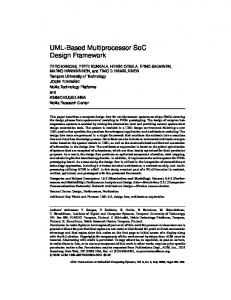
Fig. 1.

Modeling of the heat transfer inside the MPSoC

([14], [19]), to make thermal simulation faster. We present a thorough theoretical study of state-of-the-art thermal simulators to identify the Pareto points (temperature estimation time vs. accuracy) of various ODE solvers. Second, we design a scalable thermal simulator infrastructure, which identifies the optimal thermal modeling parameters for a given set of design constraints such as MPSoC floorplan granularity or desired thermal simulation time. The parameters used in the optimization flow are the order of the ODE solver, the number of cells used to model a floorplan, the simulation time step and other matrix-related parameters. Each set of simulation parameters provided by our thermal simulator infrastructure is associated with a thermal simulation method that has the shortest simulation time for a certain accuracy (or the highest accuracy for the given simulation time). Our experimental setup is based on Sun’s UltraSPARC T1 [8], and we utilize real-life workload traces ranging from webserver to multimedia benchmarks [18]. The results validate the benefits of our adaptive ODE thermal simulation infrastructure for a number of cases of operating conditions and accuracy requirements. The experiments show that our simulation infrastructure achieves up to 6× higher thermal estimation accuracy, and 70% faster simulation when compared to stateof-the-art MPSoC thermal simulators. The paper is organized as follows. Section 2 discusses the related work. In Section 3, our thermal simulation model is presented, and a matrix representation that can utilize first, second and fourth order solvers is proposed. Section 4 describes our experimental set-up, and analyzes the modeling parameters that affect the accuracy and speed of thermal simulation, identifying trade-offs between these design metrics for various ODEs. Section 5 describes our methodology for designing an optimal thermal simulation framework, and evaluates its performance based on a commercial 8-core. Finally, in Section 6 we present the main conclusions of this work.

II. R ELATED W ORK Thermal modeling and simulation at various levels of abstraction have been hot topics over the past years [1]-[5]. In [5], a thermal/power model for superscalar architectures is presented. Various abstraction levels have been used to model MPSoC temperature, such as finite element [3] and Greenfunction [4]. HotSpot [5] and the Forward Euler (FE)-based emulator [16] model the MPSoC as a network of thermal resistances and capacitances, and solve the automated model using an ODE solver. Thermal management techniques received a lot of attention recently due to the collateral effect of increasing power density. Dynamic techniques to manage thermal hot spots have been first introduced by Brooks et al. [12]. In [6] and [15], a significant reduction in localized hot spots has been obtained using thread migration techniques. Temperature-aware scheduling for MPSoCs has been presented in [18], [19]. In [14], the authors solve the optimum frequency assignment problem under thermal constraints using convex optimization and an approximation of the heat flow equation based on an FE model for rapid thermal behavior estimation. However, this speed-up has a significant loss in accuracy due to the linearization of the thermal conductance coefficient of the materials. To the best of our knowledge, a thermal simulation tool that is able to automatically choose its simulation parameters according to user accuracy and desired simulation time constraints has not been proposed before. In addition to providing an automated way to select the optimum simulation method, we present a detailed study on how various parameters (grid granularity, simulation step size, order of the ODE solver or matrix update rate) affect the accuracy and the computational complexity of the MPSoC thermal simulator. III. T HERMAL S IMULATION M ODEL In this section our thermal simulation model is described. After describing the heat propagation model, we introduce a matrix-based state-space representation suitable for various ODE solvers. Finally, we present a thorough theoretical analysis comparing the ODE solvers. A. Heat Propagation Model Similar to previous work [16], we have used two layers to model the MPSoC: the silicon layer and the heat spreading copper layer. The chip floorplan has been divided into grid cells with cubic shape. Each functional unit in the floorplan can be represented by one or more thermal cells in the silicon layer. The thermal model is formed considering the heat conductances G and capacitances C of the cells ([16],[5]). The heat flow is then modeled by a differential equation solving the resistance and capacitance network. The thermal behavior of the MPSoC is computed through the interaction of multiple discrete-time differential equations interacting with each other. A graphical representation is presented in Figure 1. In Figure 1, the gray and brown blocks represent the silicon and copper layer, respectively. The ambient temperature is modeled as a layer with uniform temperature and infinite thermal capacity. The red mark inside the silicon cell represents the cell’s power dissipation. At any moment in time, the temperature change of each block due to its neighbors is given by the temperature difference between the two blocks, multiplied by the constant that labels each pair of arrows. Since the heat propagation inside MPSoCs is a non-linear process, all coefficients inside the arrows are temperature-dependent in our model. The direction of the arrow identifies the sign of the temperature change. For example, the temperature change of cell Si−0 due to cell Si−1

is given by −(X(Si−0 ) − X(Si−1 )) · Ksi−si , where X(n) is the temperature of cell n and Ksi−si is a multiplicative constant. The temperature increase of cell Si−0 due to power dissipation is proportional to αth power of frequency, f α . The coefficient α expresses the dependence between the frequency and the power dissipated into a core. If α = 1, we have a linear dependence of power to frequency (i.e., as in frequency scaling) while if 1 < α ≤ 2 we obtain a quadratic or subquadratic dependence (i.e., voltage and frequency scaling) [14]. B. First Order ODE Solvers A first order ODE solver is the simplest and fastest solver for solving the complex system of differential equations modeling the MPSoC. Because of its simplicity, it has been used by many state-of-the-art thermal simulators like the earliest versions of HotSpot [5] or real-time thermal emulation frameworks targeting embedded SoCs [16]. Furthermore, it has been utilized by state-of-the-art thermal management policies for fast estimation of temperature on the MPSoC [14], [19]. The Forward Euler FE method is described by Eqn. 1: ¯ ∂X(t) ¯¯ (1) Xn+1 = Xn + ∆t · ∂t ¯ t=tn

where Xn and Xn+1 are the vectors containing the temperature of any thermal cell composing the MPSoC respectively ¯ at ∂X(t) ¯ time n and n+1. ∆t is the simulation step size and ∂t ¯ t=tn is the vector containing the temperature rate of change at time n. By using the model represented in Figure 1, the last term in Eqn.1 equals to: ¯ ∂X(t) ¯¯ = A0 (tn ) · Xn + B 0 · Un + W 0 (2) ∂t ¯ t=tn

where matrix A0 (tn ) expresses the part of the on-chip temperature spreading process that depends only on the cell’s temperature. This equation basically expresses all arrows of Fig. 1 in the matrix form except Kcu−RT , which needs to be 0 modeled separately. Matrix B’ is a matrix where Bi,j contains the conversion factor between the power assigned to functional unit j and the temperature increase in cell i. Matrices A0 (tn ) and B’ contain the system dynamics that depend entirely on the current state and on the given power assignment vector Un . The part of the dynamic system that is not controllable by the input vector, such as the heat dissipation of the copper layer due to room temperature, is expressed by vector W’. Then, by substituting 2 into 1, Eqn. 3 is obtained: Xn+1 = A(tn ) · Xn + B · Un + W

(3)

A(tn ) = I + ∆t A0 (tn ) B = ∆t B 0 W = ∆t W 0

(4) (5) (6)

where:

The equation above is a time-varying state-space representation modeling the thermal behavior of the MPSoC using a first order ODE solver. The computation here is simple and requires only a matrix multiplication. An important property of a solver is its “stability”. A solver is called numerically stable if an error does not exponentially grow during the calculation of the final solution. The FE method has potential stability problems when the chosen time-step for the thermal simulations is large, as shown in the literature [14], [16], which will be explored and addressed in this paper.

A first order ODE method that is unconditionally stable is the Backward Euler (BE) method. This integration algorithm ensures that the accuracy error does not grow exponentially over time for any simulation step size. The Backward Euler method is described by Eqn. 7: ¯ ∂X(t) ¯¯ Xn+1 = Xn + ∆t · (7) ∂t ¯t=tn+1 Assuming A0 (tn ) ' A0 (tn+1 ), and using Eqn. 8: ¯ ∂X(t) ¯¯ = A0 (tn+1 ) · Xn+1 + B 0 · Un + W 0 ∂t ¯t=tn+1

(8)

we can obtain Eqn. 9 in a discrete-time domain: Xn+1 = A(tn ) · Xn + B(tn ) · Un + W (tn ) where: A(tn ) = [I − ∆t A0 (tn )]−1 B(tn ) = [I − ∆t A0 (tn )]−1 ∆t B 0 W (tn ) = [I − ∆t A0 (tn )]−1 ∆t W 0

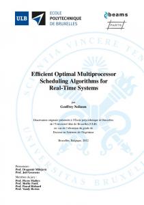
Fig. 2.

(9)

(10) (11) (12)

This method achieves unconditional stability at the cost of a significant increase in computational complexity with respect to the FE algorithm. The most costly computational requirement for the BE method is the inverse matrix computation. It has been shown in the literature [16],[5] that the accuracy of both first order methods is O(∆2t ) [20]. C. Second Order ODE Solvers As a representative example of second order solvers, we analyze the Crank-Nicholson (CN) method. This integration algorithm combines FE with BE to obtain a second order method due to cancellation of the error terms. CN method reaches an accuracy of O(∆2t ). This method can be described using Eqn. 13: " # ¯ ¯ ∂X(t) ¯¯ ∆t ∂X(t) ¯¯ Xn+1 = Xn + · + (13) 2 ∂t ¯t=tn ∂t ¯t=tn+1

Floorplan model of Sun Niagara MPSoC.

D. Multi-Step Fourth Order ODE Solver Numerical ODE solution methods, start from an initial point and take a small step in time to find the next solution point. This process continues with subsequent steps to map out the solution. Single-step methods (such as Euler’s method) refer to only one previous point and its derivative to determine the current value. Multi-step methods take several intermediate points within every simulation step to obtain a higher order method. This way, they increase the accuracy of the approximation of the derivatives by using a linear combination of these internal additional points. A multi-step solver has been embedded in the last release of HotSpot [5]. One particular subgroup of this family of multi-step solvers is the Runge-Kutta method, which includes a fourth order solver (RK4). The algorithm that we use for implementing the RK4 solver employs a FE method to compute derivatives at the internal points. By using the model represented in Figure 1, this method is described by following equations:

Assuming A0 (tn ) ' A0 (tn+1 ), and using Eqn. 2 and 8, we obtain:

k1 = ∆t · [A0 (tn ) · Xn + B 0 · Un + W 0 ] (18) k2 = ∆t · [A0 (tn+0.5 )(Xn + 0.5 · k1) + B 0 · Un + W 0 ] (19) 0 0 k3 = ∆t · [A (tn+0.5 )(Xn + 0.5 · k2) + B · Un + W 0 ] (20) 0 0 0 k4 = ∆t · [A (tn+1 )(Xn + k3) + B · Un + W ] (21) 1 (22) Xn+1 = Xn + · (k1 + 2k2 + 2k3 + k4) 6 Assuming A0 (tn ) ' A0 (tn+0.5 ) ' A0 (tn+1 ), we obtain:

Xn+1 = A(tn ) · Xn + B(tn ) · Un + W (tn )

Xn+1 = A(tn ) · Xn + B(tn ) · Un + W (tn )

(14)

where: A(tn ) = [I − 0.5 · ∆t A0 (tn )]−1 · [I + 0.5 · ∆t A0 (tn )] (15) B(tn ) = [I − 0.5 · ∆t A0 (tn )]−1 · ∆t B 0 (16) 0 −1 0 W (tn ) = [I − 0.5 · ∆t A (tn )] · ∆t W (17) As a matter of fact, higher model orders have higher computation complexity. On the other hand, the CN method is also unconditionally stable and has a higher accuracy in comparison to first order solvers when larger simulation timesteps are used. The accuracy of such second order methods can reach O(∆3t ) [20].

(23)

where: F = ∆t A0 (tn ) (24) 1 A(tn ) = I + [6F + 3F 2 + F 3 + 0.25F 4 ] (25) 6 1 B(tn ) = ∆t · [I + (3F + F 2 + 0.25F 3 )] · B 0 (26) 6 1 (27) W (tn ) = ∆t · [I + (3F + F 2 + 0.25F 3 )] · W 0 6 Note that this method does not require the inverse matrix computation. In addition, like FE, this method is not unconditionally stable, since RK4 method uses the FE for computing the rate of change of the temperature function in the internal

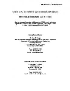
−2

10

theoretical experimental

−3

simulation step size [s]

10

Fig. 3.

Circuit for the determination of ∆Tcs and ∆Tss .

point, and hence inherits its stability properties. The theoretical accuracy of this multi-step fourth order method can reach O(∆5t ) [20]. IV. T HERMAL S IMULATOR A NALYSIS In this section we provide a theoretical analysis about the effects of the parameters in the ODE solvers on the speed and the accuracy of simulation results. Then, we provide an experimental validation with our 8-core MPSoC case study. A. Experimental Methodology Our experimental setup is based on the 8-core UltraSPARC T1 (Niagara-1) architecture from Sun Microsystems [8]. Its floorplan is shown in Figure 2. In the thermal model, we use a baseline modeling granularity of grid cells with 1mm side each, and the values regarding thermal resistance, silicon thickness and copper layer thickness have been derived from [17] and [8]. We utilize real-life workloads which were ran on an UltraSPARC T1 chip (ranging from web-server to playing multimedia) [18]. Using the utilization of cores, we derived the power traces based on the average power values reported in [8]. In all of the results for UltraSPARC T1, we display the average gains in accuracy and speed over all the benchmarks with respect to the state-of-the-art thermal simulators. B. Stability Analysis Explicit integration methods where the inverse matrix calculation is not employed suffer from a potential instability problem. Instability means that the integration error can grow exponentially at every simulation step. This issue occurs when the simulation time step is bigger or comparable to the inverse of the maximum absolute temperature rate of change of the MPSoC [20]. The maximum allowable simulation step size ∆tmax is then given by the following equation: 1 ¯ ¯ ∆tmax ≈ (28) ¯ ∂X(t) ¯ max ¯ ∂t ¯ In this section our goal is to find the maximum allowable simulation step size that avoids instability problems in the solver, assuming a worst-case scenario. According to our analysis, based on the model shown in Figure 1, the highest worst case temperature rate of change in cell Si−0 occurs when the following conditions are true: 1) Si−0 is at room temperature 2) Si−0 has the highest power dissipated per cell Pmax 3) Between Si−0 and Cu−0 , there exists the maximum temperature difference possible, ∆Tcs . 4) Between Si−0 and neighboring cells, there exists the maximum temperature difference possible, ∆Tss .

−4

10

−5

10

−6

10

0

10

1

10 block size / cell size

2

10

Fig. 4. Experimental vs. theoretical values of ∆tmax for various grid resolution values.

In this particular case, the maximum temperature rate of change is expressed by the following equation: ¯ ¯ Pmax ∆t ¯ ∂X(t) ¯ C(Si−0 ) + 4Ksi−si ∆Tss + Ksi−cu ∆Tcs ¯ ¯ = max ¯ ¯ ∂t ∆t (29) where Pmax is the the highest power dissipated per cell and C(Si−0 ) is the silicon cell thermal capacitance. To determine the value of ∆Tcs and ∆Tss , we use the circuit in Figure 3. This circuit maximizes temperature differences between the cell Si−0 and the other two cells (Si−1 and Cu−0 ) by modeling the scenario where the left half side of the cells in the floorplan are not dissipating any power and the right half side has the highest power density in the circuit. Thus, cell Si−1 is at room temperature (Tamb ) and cell Si−1 is consuming Pmax . Our target is to compute the temperature of Si−1 and Cu−0 at the equilibrium point when the highest temperature differences are present between cells. When the transient response is finalized, the result is: ∆Tss = X(Si−0 ) − X(Si−1 ) = X(Si−0 ) − Tamb

(30)

where X(j) is the temperature of cell j. According to preceding equations, to solve equation 29 we need to determine the temperature value of cells Si−0 . By analyzing and solving the circuit in Figure 3, we obtain: ∆Tss =

Pmax ∆t C(Si−0 ) (kcu−si

+ kcu−RT )

kcu−si ksi−si + kcu−RT (ksi−cu + ksi−si )

(31)

To determine the value of ∆Tcs , a different scenario needs to be considered. The scenario assumes that all silicon cells are consuming Pmax . The circuit is equivalent to the previous one in Figure 3, but this time without the arrow Ksi−si or the cell Si−1 . In this case, at the equilibrium, the following equation holds: ∆Tcs = X(Si−0 ) − X(Cu−0 )

(32)

By solving the previously described network, we obtain: ∆Tcs =

Pmax ∆t ksi−cu C(Si−0 )

(33)

Then, by substituting Eqn. 33, 31 and 29 into 28, we are able to compute ∆tmax . The resulting function is a highly non-linear

0

0

10

10

FE BE CN RK4

−1

10

−2

−1

max abs error [°C]

max abs error [°C]

10

−2

10

10

−3

10

−4

10

FE BE CN RK4

−5

10

−6

−3

10

1

1.5

Fig. 5.

2

2.5 3 3.5 block size / cell size

4

4.5

5

Accuracy vs. grid resolution of the floorplan.

function that depends on parameters such as MPSoC thermal profile, thermal cell size and dimensions of the MPSoC. In addition to the theoretical derivations, we simulated the 8-core MPSoC shown in Figure 2 using an explicit solver for various simulation step sizes (∆t ). We then identified ∆tmax as the largest ∆t value for which the integration method was working without getting unstable. We repeated the simulation for various grid resolution values. The comparisons between the theoretical and the experimental results are shown in Figure 4. Results show that the theoretical analysis is in line with the experimental simulations, as both set of results have the same trends and the difference of values is very small. The reason of the small difference is that worst case scenario assumptions make our theoretical result more conservative— i.e., ∆t max is 7% lower in the 8-core case study. Note that the theoretical derivation using Eqn. 33, 31, 29 and 28 is much faster to compute than performing an experimental derivation of ∆tmax . C. Cell Size Influence The cell size is the parameter that mostly affects the speed of the simulation. The computational complexity Nop is related to the grid granularity according to following equation: ¶2 µ block size (34) Nop = N0 · cell size where N0 is the computational complexity to process the floorplan using a cell size equal to the smallest functional block of the MPSoC. As shown in Eqn. 34, the computational complexity increases quadratically with a linear increase in the grid resolution. Figure 5 shows the accuracy of the thermal model for the various solvers we have discussed. As Figure 5 shows, with a high simulator order, the advantage of increasing the grid resolution is more obvious than the advantage observed for low-order simulators. In fact, for low accuracy solvers (such as FE or BE), the increase in accuracy is almost irrelevant considering the quadratic increase in computational complexity. D. Simulation Time Step In the previous section, we determined the value of ∆tmax . For ∆t > ∆tmax , explicit methods like the FE or the RK4

10

−5

−4

10

10 simulation time step [s]

Fig. 6.

−3

10

Accuracy vs. simulation time step ∆t .

are unstable. On the other hand, if the simulation time step is reduced, the explicit methods obtain an increase in accuracy, but at a higher computational complexity. The computational complexity Nop is related to the time step size ∆t , as shown µ ¶ in equation 35: ∆t0 Nop = N0 · (35) ∆t where N0 is the computational complexity using a step size equal to ∆t0 . The computational complexity is inversely proportional to ∆t . Figure 6 shows the accuracy change with respect to simulation step size. The effect of decreasing ∆t is visible for all the solvers. In addition, the cost in terms of computational complexity is relatively small with respect to the gain in accuracy. We also observe that usually more than one solver can meet the given error limit. For example, to achieve a desired maximum error of 10−2 ◦ C, the first order solver requires ∆t ' 6 · 10−5 , the second order solver requires ∆t ' 5 · 10−4 , and the fourth order solver requires ∆t ' 10−3 . The method we present in Section 5 automatically identifies which option provides the fastest simulation result, according to the properties of the particular MPSoC architecture. E. Inverse Matrix Calculation Period Another parameter that influences the accuracy / simulation time trade-off is the matrix calculation period (TM C ). This is the time that passes between two consecutive computations of the matrices A(tn ), B(tn ) and W (tn ). The challenge is that, these matrices are temperature dependent and they change over time during the runtime operation of the MPSoC. If the matrices are not computed sufficiently often, this can reduce accuracy. Figure 7 quantifies this error for different solvers and TM C values. As Figure 7 shows, for higher order solvers, reducing TM C becomes more beneficial than reducing TM C for low-order solvers. For low accuracy solvers, the increase of accuracy is not high enough to justify the increase in computational complexity. V. O PTIMAL T HERMAL S IMULATOR In the previous sections we analyzed state-of-the-art thermal simulators and we have proposed a generic way to represent all of them using a matrix-based state space representation.

0

10

FE BE CN RK4

max abs error [°C]

−1

10

−2

10

−3

10

0

0.005

Fig. 7.

0.01 0.015 invert matrix calculation period [s]

0.02

0.025

Accuracy vs. matrix calculation period.

Fig. 9.

Fig. 8.

Thermal simulator design flow

Parameters affecting the accuracy and the speed of the simulation have been analyzed both theoretically and experimentally. This section presents a design flow that determines the “best” thermal simulator for the desired simulation speed/accuracy trade-off on a given MPSoC. The proposed methodology exploits the previously derived results for the various simulation methods. The block diagram of the design flow is shown in Figure 8. The design flow has the following as input parameters: MPSoC floorplan, power traces for the functional units (optional), desired simulation accuracy and simulation speed. The flow produces two outputs: 1) The state-space representation of the chip thermal profile (see Section 3). This output is also useful for the thermal management policies that require a model of the MPSoC to perform optimizations. 2) The design of a thermal simulator. This design is a set of choices regarding the order of the ODE solver, the simulation time step, and the parameters described in Section IV to maximize the simulation speed for a given accuracy.

Design space exploration using our adaptive thermal simulator

The design of the adaptive thermal simulator is composed by three main steps. The first one performs a pre-processing of input parameters. It computes the maximum allowable ∆tmax by using Eqn. 33, 31, 29 and 28. Then, it simulates the thermal behavior of the MPSoC by using randomly generated power traces or real-life power traces. This simulation takes a short time, and is done by using a coarse-grid granularity. More specifically, ∆tmax is used as simulation time step and the selected grid granularity is equal to the dimension of the smallest functional block of the floorplan. In our case study, we simulated the system for a total simulation time of 100ms, and the simulation was repeated for all the solvers (FE, BE, CN and RK4). The goal of this pre-processing phase is to identify the order of the solver and the order of magnitude of the parameters that will maximize the performance of our solver for the given constraints. For this reason there is no need to perform thermal simulations with higher accuracy (and longer simulation time). The second phase performs a design space exploration in the range of values identified by the pre-processing phase. This phase varies all parameters by a few multiplicative factors and simulates the MPSoC for a longer time. Since matrices used by the solvers are temperature dependent, the simulation has to be long enough to generate temperature differences in the MPSoC thermal profile, to make the position of each Pareto point (shown in Figure 9) more reliable. More specifically, in the 8-core case study, we simulated the overall system for 10 seconds for all the combinations of the following parameters: two grid granularity values (block size/cell size = 1; 2), three step size values (∆t = ∆tmax ; ∆tmax /2; ∆tmax /4), and three values of matrix calculation period (TM C = ∆t ; 5∆t ; 9∆t ). To measure the accuracy error, the 4th order ODE solver with a small simulation time step and a high grid granularity is used as the baseline. The last post-processing step of the design phase creates the two outputs in Figure 8 with the optimum parameters, as discussed in the next section. A. Case Study This section performs an experimental validation of the method proposed in the previous section. The calculation of ∆tmax for different grid resolutions has already been shown in

simulation parameters considering the desired constraints for a given MPSoC architecture. We have used the optimal thermal simulation framework for exploring the existing trade-offs of accuracy and simulation speed in thermal modeling for reallife MPSoC designs. The experimental results on an 8-core MPSoC showed that our adaptive thermal simulation achieves significant gains in accuracy (up to 6×) and speed (up to 70%) with respect to state-of-the-art thermal simulators. R EFERENCES

Fig. 10. Normalized comparison of the proposed method (accuracy=3 · 10−3 ◦ C) with RK4-based thermal simulators (as HotSpot) and (FE)-based thermal simulators.

Figure 4. Following the proposed design method, we simulate the system for a very short time (100ms) with ∆t = 3E − 3s and a coarse-grid resolution with the block size to cell size ratio equal to 1. At this point we identify the order of the solver, and the proposed simulator design flow automatically refines our simulation until we obtain the desired optimum point in the design space. We simulated the case study for the parameters described in previous sections for all the simulators (FE, BE, CN, RK4). Results are shown in Figure 9. The optimum configurations of parameters (or Pareto points) provide the highest accuracy for a given simulation speed or vice versa. These configurations are automatically selected by our simulation framework according to the required accuracy or simulation speed for the given MPSoC design. Once these Pareto points in the design space are computed, our thermal simulator design can select the one closer to the input constraints specified. In this regard, Figure 10 compares the speed and the accuracy of the proposed method with stateof-the-art-thermal simulators like HotSpot [5] and the FEbased thermal simulator presented in [16]. All three groups of results (Proposed method, HotSpot, FE-based simulator) have error values with respect to a 4th order ODE solver with a small simulation time step and a high grid granularity. The time spent for the derivation in the proposed method of the optimal simulation parameters has been taken into account. The simulation time step is constant in both implementations. These results indicate that our adaptive simulation framework, which utilizes various ODE methods, can improve the simulation speed up to 70% with respect to HotSpot, while resulting in 6× higher accuracy. VI. C ONCLUSIONS Development of efficient thermal management strategies for MPSoCs relies on fast and accurate thermal modeling tools. This paper advances state-of-the-art temperature-aware system design in two main directions. First, we have presented a novel state-space representation that can be used to combine various ODE solvers or to choose the best fitting solver, without the need for adjusting the representation according to the solver. The second contribution is the definition of an optimal thermal simulation framework that uses this novel representation, and selects the best solver and the optimum

[1] J. Li et al.,Power-performance implications of thread-level parallelism in chip multiprocessors, Proc. ISPASS, 2005. [2] J. Deeney,Thermal modeling and measurement of large high power silicon devices with asymmetric power distribution, Proc. ISM, 2002. [3] B. Goplen et al.,Efficient thermal placement of standard cells in 3D ICs using a force directed approach, Proc. ICCAD 2003. [4] Y. Zhan et al.,Fast computation of the temperature distribution in VLSI chips using the discrete cosine transform and table look-up, Proc. ASPDAC 2005. [5] K. Skadron et al.,Temperature-aware microarchitecture: Modeling and implementation, TACO, 2004. [6] P. Chaparro, J. Gonzalez, G. Magklis, Q. Cai, and A. Gonzalez. , Understanding the thermal implications of multi-core architectures., IEEE TPDS, 2007. [7] D. Pham et al.,Design and Implementation of a First-Generation Cell Processor., Proc. ISSCC, 2005. [8] P. Kongetira et al.,Niagara: A 32-way multithreaded SPARC processor., IEEE Micro, 2005. [9] Tilera Corporation,Tilera’s 64-core architecture, www.tilera.com/products/processors.php, 2007. [10] O. Semenov et al.,Impact of self-heating effect on long-term reliability and performance degradation in CMOS circuits, IEEE T-D&M, 2006. [11] S. Borkar,Design challenges of technology scaling, IEEE Micro, 1999. [12] D. Brooks et al.,Dynamic thermal management for high-performance microprocessors, Proc. HPCA, 2001. [13] C J. Hughes et al.,Saving energy with architectural and frequency adaptations for multimedia applications, Proc MICRO, 2001. [14] S.Murali et al.,Temperature Control of High Performance Multicore Platforms Using Convex Optimization, Proc. DATE, 2008. [15] J. Donald et al.,Techniques for multi-core thermal management: Classif. and new exploration, Proc. ISCA, 2006. [16] D. Atienza et al.,HW-SW Emulation Framework for Temperature-Aware Design in MPSoCs, ACM TODAES, 2007. [17] M.-N. Sabry,High-precision compact-thermal models. IEEE Transactions on Components and Packaging Technologies, 2005. [18] A. K. Coskun, et al., Static and Dynamic Temperature-Aware Scheduling for Multiprocessor SoCs, IEEE Transactions on VLSI, vol.16 no.9, pp. 1127-1140, Sept. 2008. [19] F. Zanini, et al., A Control Theory Approach for Thermal Balancing of MPSoC, Proc. ASP-DAC, 2009. [20] Burden Richard L, et al., Numerical Analysis, 7th ed. Belmont, CA: Brooks Cole, 2000.