Published by Elsevier Science Ltd. All rights reserved 12th European Conference on Earthquake Engineering Paper Reference 467 (quote when citing this paper)
OPTIMAL PROBABILISTIC SEISMIC DEMAND MODELS FOR TYPICAL HIGHWAY OVERPASS BRIDGES K Mackie1, B Stojadinovic1 1
University of California, Berkeley, Dept. of Civil & Env. Engineering, 721 Davis Hall #1710, Berkeley, CA 94720-1710, email
[email protected]
ABSTRACT Performance-based seismic design is founded on our ability to evaluate the performance of a structure in a given seismic hazard environment. The Pacific Earthquake Engineering Research Center (PEER) is developing such a probability-based performance framework, one component of which is a seismic demand model. While probabilistic seismic hazard models have been developed before, rigorous probabilistic demand models do not exist. The objective of this paper is the development of an optimal probabilistic seismic demand model for typical highway overpass bridges. This demand model relates ground motion Intensity Measures, such as spectral displacement, to bridge Demand Parameters, such as column curvature ductility or drift ratio. An optimal model is defined herein as practical, sufficient, effective, and efficient. A parametric finite element model, representing an entire bridge portfolio, was used to compute values of bridge-specific Demand Parameters. Probabilistic seismic demand models were formulated by statistical analysis of the data produced during time history analyses of each bridge in the bridge portfolio under all ground motions. A representative relation between chosen Intensity and Demand Measure pairs forms the basis of the demand models presented.
KEYWORDS bridges, performance-based design, earthquake intensity measures, structural demand parameters, probabilistic seismic demand model
INTRODUCTION Performance-based earthquake engineering (PBEE) describes a quantitative means for designers of structures to achieve predetermined performance levels or objectives. Traditionally, performance-based design frameworks have addressed only the probabilistic evaluation of seismic hazards, as in FEMA-273 [1] and Vision 2000 [2]. The subsequent graduated arrays of performance levels are based on deterministic estimates of structural performance. This deficiency has been confronted recently in the SAC Steel Project [3], which provides a means for considering uncertainties simultaneously in both the demand and capacity, in a probabilistic manner.
In the thrust to achieve a consistent probability-based framework that is significantly more general than that of the SAC project, the Pacific Earthquake Engineering Research Center (PEER) is developing a probabilistic framework for performance-based design and evaluation. Performance objectives are defined in terms of annual probabilities of socioeconomic Decision Variables (DV) being exceeded. While useful to owners and designers, such an outcome is de-aggregated into several interim probabilistic models to address the problem rigorously. These involve global or component Damage Measures (DM > y), structural Engineering Demand Parameters (EDP > x), and seismic hazard Intensity Measures (IM > w). Thus, the mean annual frequency (MAF) of a DV exceeding limit value z is [4]:
ν DV ( z ) = ∫ ∫ ∫ GDV | DM ( z | y) | dGDM | EDP ( y | x ) || dGEDP| IM ( x | w ) || dλ IM ( w ) |
(1)
y x w
The de-aggregation of Eq 1 is possible only when the components are mutually independent. The intermediate variables (DM, EDP, IM) are chosen such that probability conditioning is not carried over from one model to the next. Additionally, the uncertainties over the full range of model variables needs to be systematically addressed and propagated, making the selection of each interim model critical to the process. This paper addresses the choice of interim variables IM and EDP when selecting an optimal probabilistic seismic demand model in Eq 1, specifically applied for highway overpass bridge systems.
OPTIMAL MODELS Optimal is defined henceforth as being practical, sufficient, effective, and efficient. An IMEDP pair is practical if it has some direct correlation to known engineering quantities. Specifically, IMs derived from known ground motion parameters and EDPs from resulting nonlinear analysis. Correlation between analytical models and experimental data lend further practicality to the EDPs of the demand model. As discussed in Eq 1, the PEER performance-based design framework achieves deaggregation of the hazard and demand model, if and only if the IM-EDP pair does not have a statistical dependence on ground motion characteristics, such as magnitude and distance. Such demand models with no conditional dependence are termed sufficient. Sufficiency is further investigated in the sample models presented below. Effectiveness of a demand model is determined by the ability to evaluate Eq 1 in a closed form. For this to be accomplished, it is assumed the EDPs follow a log-normal distribution [5]. Thus an equation describing the demand model can be written as
EDP = a( IM )b
(2)
to which a linear regression in log-log space can be applied to determine the coefficients. Demand models lending themselves to this form allow closed form integration of Eq 1 and casting the entire framework in an LRFD type format [4]. An example of such an implementation is the SAC project [13,3] for steel moment frames. Efficiency is the amount of variability of an EDP given an IM. Specifically, linear regression provides constants in Eq 2, as well as the distribution of data about the linear, or piecewise linear, fit. The measure used to evaluate efficiency is the dispersion (Eq 3), defined as the standard deviation of the logarithm of the demand model residuals [5]. An efficient demand
model requires a smaller number of nonlinear time-history analyses to achieve a desired level of confidence. In general, dispersion is a measure of randomness, or aleatory uncertainty, but is not the only source of uncertainty. Not investigated in this study is the epistemic uncertainty derived from such issues as modelling, nonlinearity, approximate analysis methods, and limited number of ground motions considered [13].
PROBABILISTIC SEISMIC DEMAND MODEL The Probabilistic Seismic Demand Model (PSDM) formulated herein is the outcome from Probabilistic Seismic Demand Analysis (PSDA). PSDA has been previously used [5] to couple Probabilistic Seismic Hazard Analysis (PSHA) with demand predictions from finite element analysis. This is done in order to estimate the mean annual frequency of exceeding a given demand, and results in a structural demand hazard curve [6] in a conjectured hazard environment. This integration is not explicitly performed herein, rather, the demand model is emphasized. The procedure used to formulate the PSDMs of interest involves five steps. First, a set of ground motions, representative of regional seismic hazard, is selected or synthesized. Instrumental in selecting motions is categorizing them according to computable Intensity Measures descriptive of their content and intensity. Second, the class of structures to be investigated is defined. Associated with this class are a suite of Engineering Demand Parameters which can be measured during analysis to assess structural performance under the considered motions. Third, a nonlinear finite element analysis model is generated to model the class of structures selected. Fourth, nonlinear dynamic analyses are performed until all motions and structure model combinations have been exhausted. Fifth, a demand model is formulated between resulting ground motion Intensity Measures and structural Demand Parameters. PSDA Ground Motions The PSDA method used herein to formulate the PSDMs involves the ground motion bin approach only. The bin approach, proposed and used by Shome and Cornell [5], is used to subdivide ground motions into imaginary bins based on magnitude (Mw), closest distance (R), and local soil type. The use of magnitude and distance allows parallels between standard attenuation relationships and existing PSHA. Advantages of the bin approach include the ability to assess the effect of generalized earthquake characteristics on structural demands. Second, the use of bins can be substantial in limiting the number of ground motions selected for analysis. Given a log-normal distribution of Demand Parameters [5], the number of records required to attain a desired level of confidence is proportional to the square of the dispersion in the demand model. The bins in this study are delineated at a magnitude of 6.5 and a distance of 30 km. Four bins with 20 ground motions each were obtained from the PEER Strong Motion Database (peer.berkeley.edu/smcat), and are characteristic of non-near-field motions (R > 15 km) recorded in California. The specific records selected are the same as those used by Krawinkler [7,8] in companion building research in PEER. These motions were all scaled by a factor of 2 (amplitude scaling only), and the sampling period reduced to 0.02 seconds. This reduced the number of dynamic time steps required, while having little effect on the primarily first-mode dominated bridge system. All three ground motion components were applied to the model. As the intention of the bin strategy is
to vary the seismic demand, not capture near-field or directivity effects, the records were not rotated prior to use in order to maintain orthogonality of the original motion. PSDA Class of Structures In this study, typical new California highway overpass bridges are selected as the class of structures. The class is defined by geometry, components, and methods of design. Ideally, each of these can be investigated in a parameter sensitivity study from the resulting PSDMs. The bridges presented in this paper are designed according to Caltrans Bridge Design Specification and Seismic Design Criteria [9] for reinforced concrete bridges. Consistent with the displacement-based design approach outlined by Caltrans, the assumption is made regarding new design methods and techniques, such that columns develop plastic hinges in flexure rather than experience shear failure. Configurations in this study are limited to two-equal-span overpasses including abutments on either end. Common to all bridges is a single column bent anchored below grade by a Type I integral pile foundation. Ten design parameters were initially selected to describe variations in the aforementioned bridge. They are detailed in [12]. To assess performance, a series of displacement and force based demand parameters was selected and calculated for every bridge analysis. PSDA Model and Analysis The PEER OpenSees (www.opensees.org) platform was selected as the nonlinear finite element engine for PSDA. Bridge columns and pile shafts are modeled using threedimensional flexibility-based beam-column elements with fiber cross-sections. This element is limited to axial-flexural interaction. P-∆ effects were included for the column, but no other methods of softening were incorporated into the model, eliminating the evaluation of the collapse state. The circular column cross-sections have perimeter longitudinal reinforcing bars and spiral confinement. Soil-structure interaction was modeled using bilinear p-y springs at varying depths over the length of the pile shafts. The p-y spring properties were determined using assumed soil parameters corresponding to USGS soil categories and recommendations from the API [10]. The bridge deck was designed as a typical Caltrans reinforced concrete box girder section for a three-lane roadway. During the nonlinear analyses, the deck was assumed to remain elastic, therefore input into the model using elastic elements and cracked stiffnesses. The modeling of abutments varies widely based on different available research, however is no less important, as the response of short- and medium-span bridges is expected to be largely dominated by abutment stiffness. In this study, simple elastic-plastic spring-gap elements were implemented. In order to maximize the column demand, the stiffnesses are set to zero, creating a roller condition at the abutments. Nonlinear models were generated for each of the 116 bridge configurations and analyzed for each ground motion. Each routine involves a static pushover analysis to determine yield values, a modal analysis to determine natural frequencies, and a dynamic time-history analysis to determine demand. From modal analysis, the first two mode shapes were practically identical for all of the considered bridges. The first mode shape is dominated by longitudinal deck motion accompanied by small deck rotations near the abutments. The second mode shape is dominated by simple transverse motion of the deck. Period details are listed in [12].
Following modal analyses, nonlinear time-history analyses were completed. The results of statistical analyses of the data in the database are shown in Figures 1 through 10 and discussed in the examples. In each of these figures, the data is plotted on a log-log scale, with the EDP on the abscissa and the IM on the ordinate. Traditional force (IM) displacement (EDP) relationships are plotted in this manner, even though the IM is still regarded as the dependent variable. PSDA Intensity Measures and Demand Parameters The final step in PSDA is to combine all the analyses of interest into PSDMs, which relate ground motion specific Intensity Measures (IM) to class-specific structural Engineering Demand Parameters (EDP). Given the wide array of IMs and EDPs for every analysis, it is critical to select an optimal PSDM. The ground motion IMs used are detailed in [12]. They range from spectral quantities, across duration and energy related quantities, to frequency content characteristics. Each IM is ground motion specific and independent of the bridge model, except for period based spectral quantities. The bridge EDPs were chosen from the PEER database of experimental results for concrete bridge components [13,14]. The database details specific discrete limit states for each of the EDPs considered. The measures range from global, such as drift ratio, to intermediate, such as cross-section curvature, to local, such as material strains. A regression analysis of the data yields linear equations of the form log( EDP) = A + B log( IM )
(3)
where A and B are the coefficients of a linear, or piecewise-linear regression in the log-log coordinate space. The dispersion values for each regression analysis, computed from the natural log of the residuals of the EDPs, are listed in each corresponding figure window. In this particular study, a bilinear least squares fit was made to all parametric models to reduce the dispersions. Each demand model is constructed in the longitudinal and the transverse direction independently.
SAMPLE OPTIMAL PSDMS Presented below is a small subset of the parametric study, focusing on the parameters that produce an optimal demand model. All of the parameters presented are in reference to a base bridge configuration. The base configuration includes two 18.2 m (60 ft) spans, a singlecolumn bent 7.6 m high (30 ft), with a 1.6 m (5.25 ft) diameter circular column, 2% longitudinal reinforcement, and 0.7% transverse reinforcement. As the bridge parameters are varied, their values relative to each other are intended to cover the complete spectrum of possible bridge designs, even if independent values are uncommon in design practice. The base bridge is on a USGS class B (NEHRP C) soil site. Only one parameter was varied from the base configuration at a time. Parameters referenced in this paper are limited to the percent of column longitudinal reinforcement and column- to superstructure-depth ratio. Given the varying engineering usefulness of each of the EDPs calculated, an optimal demand model for each was developed. Several of the computed demand parameters are mutually dependent, e.g. displacement ductility and drift ratio, and one is neglected. Residual
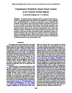
displacements yield poor IM-EDP relationships and are therefore also neglected [12]. The remaining EDPs considered can be categorized as either local, intermediate, or global. Local Demand Parameters Local demand quantities such as material stress in the column proved to be good performance indicators. Peak stress values in both steel and concrete materials were computed at the critical column cross-section. In order to maintain comparability with the other EDPs considered, a PSDM for steel stress (σ steel) is first developed using ρs (Figure 1) and D cDs (Figure 2) as the parameters of variation. These produce very efficient fits, largely due to the plateauing behaviour at high stress levels. The bilinear fits largely reflect a bilinear material stress-strain envelope when the strain is thought of as a function of earthquake intensity. In either case, stronger and stiffer bridges show trends toward reduced demand. Intensity Measure vs Damage Measure (Parameters)
Intensity Measure vs Damage Measure (Parameters)
σ=0.13, 0.16, 0.17, 0.15
σ=0.20, 0.16, 0.18, 0.18
3
Sa T1 Longitudinal (cm/s2)
10
1
Sd T1 Longitudinal (cm)
10
ρ ,ln=0.01 s ρs,ln=0.02 ρ ,ln=0.03 s ρs,ln=0.04
Dc/Ds=0.67 Dc/Ds=0.75 Dc/Ds=1 Dc/Ds=1.3
2
10 2
10 Maximum Steel Stress
Figure 1 - SdT1-σsteel, ρs sensitivity long.
1
10 Maximum Steel Stress
Figure 2 - SaT1-σsteel, DcDs sensitivity long.
While fundamental mode periods are roughly equivalent for variation of the longitudinal reinforcing ratio, the use of Sd can be confusing since changing parameters also modifies the bridge period (e.g. stiffness in the DcDs case, Figure 2). In the ρ s case (Figure 1), a line of constant intensity can be drawn across the plot to determine performance. Results indicate the use of Arias Intensity or PGV as non-period-dependent IMs yields models with dispersions approximately 50% higher. Intermediate Demand Parameters Figure 3 shows the ensuing PSDM for maximum moment in the longitudinal direction. The optimal IM for parametric variation of column diameter- to superstructure depth- ratio (DcDs) is first mode Spectral Displacement (SdT1). Spectral Displacement of the second mode period (SdT2) provides an appropriate extension of this relationship to the transverse direction (Figure 4). As would be expected, the stiffer the column is made, the more force it attracts. More flexible structures indicate higher dispersion. Results indicate the use of Arias Intensity or PGV yields models with dispersions approximately 40% higher. In addition, PGV and Arias Intensity demand models exhibit higher dispersion for stiffer structures. It should be noted that, although not investigated rigorously in this study, there is a strong sensitivity of the optimal IM-EDP pair to the period (stiffness) of the structure under consideration. This trend is exhibited between stiffer/stronger structures and the demand model dispersion values. Figures 3-6 are typical, showing reduction in dispersion as the stiffness/strength of the structure is increased through parametric variation. Some IMs are
more susceptible to this increase, specifically motion content measures such as Arias Intensity, cumulative absolute velocity (CAV), and spectral displacement. Intensity Measure vs Damage Measure (Parameters)
Intensity Measure vs Damage Measure (Parameters)
σ=0.21, 0.18, 0.15, 0.13
σ=0.24, 0.21, 0.31, 0.31
1
10
1
Sd T1 Transverse (cm)
Sd T1 Longitudinal (cm)
10
0
10
0
10
Dc/Ds=0.67 Dc/Ds=0.75 Dc/Ds=1 Dc/Ds=1.3
Dc/Ds=0.67 Dc/Ds=0.75 Dc/Ds=1 Dc/Ds=1.3
5
5
10 Maximum Moment Longitudinal
10 Maximum Moment Transverse
Figure 3 - SdT1-Moment, DcDs sensitivity long.
Figure 4 - SdT1-Moment, DcDs sensitivity trans.
Column curvature ductilities are investigated next. The most efficient and effective fits are once more obtained by using SdT1 as the IM. The PSDM varying DcDs for curvature ductility is shown in Figure 5, Sa T 1 as the IM for an example (spectral quantities can be used interchangeably). Dispersions are roughly independent of selection of either DcDs or ρs. The large period dependence of the dispersions in this model should be noted. As discussed earlier, it may be useful for the designer to consider period dependent parameters. Therefore, to eliminate Sd shifts, the use of Arias Intensity, Characteristic Intensity, or PGV as an IM increases dispersions by approximately 20%. Intensity Measure vs Damage Measure (Parameters)
Intensity Measure vs Damage Measure (Parameters)
σ=0.67, 0.50, 0.44, 0.17
σ=0.40, 0.29, 0.24, 0.15
3
3
10
Sa T1 Longitudinal (cm/s2)
2
Sa T1 Longitudinal (cm/s )
10
Dc/Ds=0.67 Dc/Ds=0.75 Dc/Ds=1 Dc/Ds=1.3
2
10
Dc/Ds=0.67 Dc/Ds=0.75 Dc/Ds=1 Dc/Ds=1.3
2
10 -1
10
0
10 Curvature Ductility Longitudinal
Figure 5 - SaT1-µφ, DcDs sensitivity long.
1
10
-1
0
10
10 Drift Ratio Longitudinal
Figure 6 - SaT1-Drift ratio, DcDs sensitivity long.
Global Demand Parameters The final PSDM developed in this paper is for longitudinal drift ratio. The optimal model is obtained by varying D cDs and again using SaT1 as the IM (Figure 6). Other possibilities include incorporating Arias Intensity, CAV, or inelastic Spectral Displacement of the first mode as the IM. These options increase dispersions approximately 33%-40%. Note the efficiency of the fit for the high stiffness parameter, DcDs =1.3.
Verifying Optimal Model From the previously discussed models, the relationship between SaT1 and longitudinal drift ratio for the column diameter (DcDs) parameter variation (Figure 6) is selected to investigate other demand model properties. As with any of the models, it is possible to generate not only the mean, but the µ ± 1σ (84th percentile) distribution stripes. This probability distribution is shown for the above example case in Figure 7. Intensity Measure vs Damage Measure (Parameters)
Residual Dependence (semilog scale)
σ=0.29, 0.15
-2 2.2 c (*E )=-24.26, -6.30, 1.28, -6.85
Drift Ratio Longitudinal residual
Sa T1 Longitudinal (cm/s2)
2
3
10
1.8 1.6 1.4 1.2 1 0.8 Dc/Ds=0.67 Dc/Ds=0.75 Dc/Ds=1 Dc/Ds=1.3
0.6 2
Dc/Ds=0.75 Dc/Ds=1.3
10
-1
0
10
10
0.4 5.8
5.9
6
6.1
Drift Ratio Longitudinal
Figure 7 - SaT1-Drift ratio, DcDs, µ±1σ
6.2 6.3 Magnitude
6.4
6.5
6.6
6.7
6.8
Figure 8 - SaT1-Drift ratio, DcDs, M dependence
Efficiency and effectiveness have already been established, however, sufficiency and practicality remain to be confirmed. The classification of practicality is, unfortunately, a subjective exercise. In the perception of the EDP holding a particular definition in the engineering sense, maximum material stress is then also practical. However, in terms of instrumentation and physical test specimens, stress by itself is an indeterminable physical quantity. A clearly practical EDP is the global drift ratio. Sufficiency is required to determine whether the total probability theorem can be used to deaggregate the various components of the PEER framework equation. This cannot be done if there are any residual dependencies on M, R, etc. Eq 4 can be used if the demand model is statistically independent, otherwise Eq 5 must be utilized, necessarily complicating evaluation of Eq 1.
ν EDP ( y) = ∫ GEDP| IM ( y | x ) | dλ IM ( x ) |
ν EDP ( y) = ∫ GEDP| IM , M , R ( y | x, M , R) | dGM , R| IM ( M , R | x ) || dλ IM ( x ) |
(4) (5)
To assess this sufficiency, regression on the IM-EDP pair residuals is performed, conditioned on M, R , and strong motion duration. The resulting sufficiency plots for the PSDM of interest are shown in Figures 8 and 9. The first takes moment magnitude (M w ) from the database of IMs and plots it versus the residual of the chosen IM-EDP fit. Similarly, the second plots residual versus closest distance (R). The slopes of the linear regression lines in the plot are shown at the top of each of the plots. Small slope values for all parameters indicate that these demand models have the sufficiency required to neglect the conditional probability as described above.
Bin dependence (LMSR -) (LMLR -.) (SMSR --) (SMLR..)
Residual Dependence (semilog scale) -2
2.2 c (*E )=0.37, 0.37, 0.24, -0.10
3
2
Sa T Longitudinal (cm/s )
1.6 1.4 1.2 1
10
1
Drift Ratio Longitudinal residual
2 1.8
0.8 Dc/Ds=0.67 Dc/Ds=0.75 Dc/Ds=1 Dc/Ds=1.3
0.6 0.4 15
20
25
30 35 Distance (km)
40
45
50
55
Figure 9 - SaT1-Drift ratio, DcDs, R dependence
Dc/Ds=0.67 Dc/Ds=0.75 Dc/Ds=1 Dc/Ds=1.3
2
10
-1
0
10
10 Drift Ratio Longitudinal
Figure 10 - SaT1-Drift ratio, DcDs , bin depend.
The use of the bin approach also needs to be evaluated to determine what, if any, bias has been introduced into the results from different bins. A seismicity plot is generated by fitting the data based on each of the four bins to the same cloud of points. The regression in this case is too scattered to show any definite trends, however, it can be noted that the higher intensity earthquakes (LMSR) produce higher demand. In order to uncouple the different design parameter variations in the seismicity plot, it is necessary to plot 16 lines, one for each of the bins and each of the design parameter values (Figure 10). To minimize the clutter, only linear fit lines are shown, the data points have been removed. In order for the model to be independent of the choice of bins, the lines of same color (corresponding to individual design parameter values) should exhibit the same slope at a given intensity level. As bins have different concentrated ranges of intensities, care should be taken not to bias the slope of the fit lines in these regions.
CONCLUSIONS This paper provides insight into the selection of an optimal demand model (PSDM) for a class of real structures, in this case typical California highway overpass bridges. Given the requirements that demand models need be practical, sufficient, effective, and efficient, the task of optimizing becomes complex. For the design parameters discussed in this paper applied to demand models in the bridge longitudinal and transverse directions, it was found that first mode spectral displacement (SdT1) is the optimal IM when coupled with a variety of EDPs. These EDPs include local measures (maximum material stresses), intermediate measures (maximum column moment), and global measures (drift ratio). With a small tradeoff in efficiency, the use of period-independent Arias Intensity as the IM is also acceptable. The PSDMs described in this paper can be used directly by designers as structural demand hazard curves. They allow assessment of design parameter variations on structural performance. Cast as a component model in a performance-based earthquake engineering framework, such as Eq 1, PSDMs provide the probabilistic relationship between ground motion IMs and structure-specific EDPs. The IM side can be coupled with hazard models and the EDPs to fragility models in order to achieve probabilities of exceedance of such economic variables such as repair cost, wherein the true value of PBEE lies.
ACKNOWLEDGEMENT The authors gratefully acknowledge support by the Earthquake Engineering Research Center s Program of the National Science Foundation under Award Number EEC-9701568 as PEER Project #312-2000 Seismic Demands for Performance-Based Seismic Design of Bridges. The authors are also grateful to Professor C. Allin Cornell and a group of his graduate students at Stanford University for enlightening discussions about PSDMs. The opinions presented in this paper are solely those of the authors and do not necessarily represent the views of the sponsors.
REFERENCES 1. Federal Emergency Management Agency (FEMA). NEHRP guidelines for the seismic rehabilitation of buildings. Rep. No. FEMA-273, Washington D.C., 1996. 2 . Structural Engineers Association of California (SEAOC). A framework for performance based design. Rep. Vision 2000, Sacramento, Calif., 1995. 3. Federal Emergency Management Agency (FEMA). Recommended Seismic Design Criteria for New Steel Moment-Frame Buildings. Rep. No. FEMA-350, Washington D.C., July 2000. 4 . Cornell CA, Krawinkler H. Progress and Challenges in Seismic Performance Assessment. PEER Center News Spring 2000; 3(2). 5. Shome N, Cornell CA. Probabilistic seismic demand analysis of nonlinear structures. Reliability of Marine Structures Rep. No. RMS-35, Dept. of Civ. and Envir. Engrg., Stanford University, Stanford, Calif., 1999. 6. Luco N, Cornell CA, Yeo GL. Annual limit-state frequencies for partially-inspected earthquake-damaged buildings. In: 8th International Conference on Structural Safety and Reliability. International Association for Structural Safety and Reliability (IASSAR), Demark, 2001, in press. 7. Gupta A, Krawinkler H. Behavior of ductile of SRMFs at various hazard levels. J. Struct. Engrg. 2000, ASCE; 126(1): 98-107. 8. Medina R, Krawinkler H, Alavi B. Seismic drift and ductility demands and their dependence on ground motions. In: US-Japan Seminar on Advanced Stability and Seismicity Concepts for Performance-Based Design of Steel and Composite Structures, Kyoto, Japan, July 23-27, 2001. 9. Caltrans. Seismic Design Criteria. California Department of Transportation, 1.1 (July 1999). 10. American Petroleum Institute (API). Recommended practice for planning, designing, and constructing fixed offshore platforms - Load and resistance factor design. Rep. No. RP2A-LRFD, Washington D.C., 1993. 11. Cornell CA, Jalayer F, Hamburger RO, Foutch DA. The probabilistic basis for the 2000 SAC/FEMA steel moment frame guidelines. Submitted to J. Struct. Engrg. 2001, ASCE. 12. Mackie K, Stojadinovic B. Probabilistic Seismic Demand Model for California Highway Bridges. J. Bridge. Engrg. Nov/Dec 2001, ASCE; 6(6): 468-481. 13. Hose Y, Silva P, Seible F. Development of a performance evaluation database for concrete bridge components and systems under simulated seismic loads. Earthquake Spectra 2000; 16(2): 413-442. 14. University of California, San Diego. The UCSD/PEER performance library for concrete bridge components, sub-assemblages, and systems under simulated seismic loads. http://www.structures.ucsd.edu/PEER/Capacity_Catalog/capacity_catalog.html, 1999.