Jan 13, 2014 - the dynamics of quantum Fisher information are employed as a measure to ..... So this state corresponds to the largest value of max(Fγ).
Optimal quantum parameter estimation of two interacting qubits under decoherence Zheng Qiang
arXiv:1401.2733v1 [quant-ph] 13 Jan 2014
1
1, 2
, Yao Yao 1 , Yong Li
1
Beijing Computational Science Research Center, Beijing 100084, China 2 School of Mathematics and Computer Science, Guizhou Normal University, Guiyang, 550001, China
We investigate the parameter estimation problem in a two-qubit system, in which each qubit is independently interacting with its Markovian environment. We study in detail the sensitivity of the estimation on the decoherence rate γ and the two-qubit interaction strength v. In particular, the dynamics of quantum Fisher information are employed as a measure to quantify the precision of the estimations. We find that the quantum Fisher information with respect to the decoherence rate scales like t2 /[exp(γt) − 1] and exp(−2γt) in the unitary limit and the completely decoherent limit, respectively. When we estimate the interaction strength v, the quantum Fisher information shows oscillation behavior in term of time. In addition, our results provide further evidence that the entanglement of the input state may not enhance quantum metrology. PACS numbers: 03.67.-a; 42.50.St; 42.50.Dv
I.
INTRODUCTION
Each quantum system is in contact with its environment. Understanding the dynamics of physical quantities under the effect of its decoherence environment has attracted much more interest. On a foundational level, time is a basically physical quantity. So the dynamical evolution is an important property of system, which makes the finite-time quantum quantities interesting in their own right [1]. An well-known example is that the entanglement dynamics of two qubits exhhibits entanglement sudden death [2] in the decoherent environments. The environmental noise presented in the physical system often determines the performance of quantum property. Therefore, it is important to develop methods to estimate the level of noise as precisely as possible. Determining the environmental parameters affecting a quantum system is the first step to develop means to control its spoiling effects. Except quantum process tomography [3], quantum channel estimation [4] is an efficient way to identify an unknown noise by estimating noise parameters. A general description of quantum channel estimation is as follows: for a prepared state ρ as an input of quantum channel Υθ , the channel parameters may be estimated efficiently by performing some quantum state measurements on the output state Υθ (ρ). Thus, one should seek an optimal input state ρ and/or an optimal measurement on the output state Υθ (ρ). Very recently, based on optical setup, the experimental realization of optimal estimation is reported for a Pauli noisy channel [5]. Fisher information [6] is a key quantity in classical estimation theory. Extending to quantum regime, quantum Fisher information (QFI) is also very important in quantum estimation theory and quantum information theory. QFI characterizes the sensitivity of a state with respect to changes on a parameter [8]. It is also related to Cram´ erRao inequality [7], which determines the bound of the optimal measurement. In the field of quantum estimation, the aim is to determine the value of the unknown
parameter labeling the quantum system, and the primary goal is to enhance the precision of resolution. Moreover, QFI is also closely related with other quantity, especially entanglement [9]. Previously, Huelga et. al. have discussed the optimal precision of frequency measurements in the presence of decoherence [10]. In a recent paper, a general theory for the quantum metrology of noisy systems has been proposed by Escher and co-workers [11]. More recently, the dynamics of QFI under decoherence excites wide interest. It has been shown that the evolution of QFI under decoherence for the N -qubit GHZ state shows the decay and sudden change [12]. For a spin-j system surrounded by a quantum critical Ising chain, the QFI decays almost monotonously when the environment reaches the critical point [13]. The dynamics of QFI for a qubit subject to a non-Markovian environment shows revival and retardation loss [14]. The main aim of this paper is to examine the problem of parameter estimation for two initially entangled qubits under decoherence. In particular, we focus on the dynamical evolution of quantum Fisher information. Quantum Fisher information shows the revival-like behavior in the Markovian environment when the estimated parameter is their interacting strength. This generalizes the result in Ref. [14]. We also show that quantum Fisher information can not be enhanced by the entanglement of initially mixed state. This extends the general result that the entangled states can improve the precision of parameter estimation [15, 16] from the view point of QFI dynamics.
II.
QUANTUM FISHER INFORMATION
The classical Fisher information is defined as Fθ,
c
=
P
i
∂ pi (θ)[ ∂θ ln pi (θ)]2 ,
(1)
where pi (θ) is the probability density conditioned on the fixed parameter θ with measurement outcome {xi } for a
2
F
γ
100
FIG. 1: Schematic diagrams of the parameter estimation adopted in this paper. Two qubits A and B couple to each other by the interaction parameter v. They also have equally local decoherent rates γ. (a) corresponds to the estimate of γ taking the two qubits as a whole, (b) corresponds to the estimate of v only using qubit B.
discrete observable X. The classical Fisher information characterizes the inverse variance of the asymptotic normality of a maximum-likelihood estimator. Extending to quantum regime, quantum Fisher information of a parameterized quantum states ρ(θ) is defined as Fθ = Tr[ρ(θ)L2 ],
(2)
where θ is the parameter to be measured, and L is the symmetric logarithmic derivative determined by dρ(θ) dθ
(3) = 12 [ρ(θ)L + Lρ(θ)]. P With the spectrum decomposition ρθ = k λk |kihk|, its QFI with respect to θ is given as [17–19] Fθ =
X (∂θ λk )2 k
λk
+2
X (λk − λk′ )2 k,k′
λk + λk′
|hk|∂θ k ′ i|2 .
(4)
Here λk > 0 and λk + λk′ > 0. The first term in Eq. (4) is just the classical Fisher information Eq. (1). Then, the second term can be considered as the quantum contribution. According to quantum Cram´ er-Rao (QCR) ˆ of any unbiased estimator inequality, the variance Var(θ) θˆ satisfies ˆ ≥ Var(θ)
1 MFθ ,
(5)
where M is the times of measurement. QCR embodies the ultimate limit to the precision of the estimate of θ. With a larger quantum Fisher information, the parameter θ can be estimated more accurately.
III.
QUANTUM FISHER INFORMATION OF TWO QUBITS A.
Model
In order to study the the precision of parameter estimation, we consider a model consisting of two identically interacting qubits A and B [20]. This simple model can make us get analytical results for the time evolution of
50 0 1 a 0.5 20 t
0 0
40
60
FIG. 2: The variation of Fγ in Eq. (14) with respect to the time t and the parameter a. Here the decoherence parameter γ = 0.1.
QFI. Each qubit is a two-level system with an excited state |ei and a ground state |gi. The interacting Hamiltonian is given by + − H = 12 v(SA SB + h.c.).
(6)
Here v denotes the interaction strength between the two qubits, Sj+ and Sj− (j=A, B) are the qubit’s raising and lowering operators, respectively. Furthermore, each qubit interacts independently with its Markovian environment. The decoherence may arise from the spontaneous emission of the excited state. The dynamics of the system can be treated by quantum Liouville equation (¯h = 1) X γj dρ(t) = −i[H, ρ]− (S + S − ρ−2Sj− ρSj+ +ρSj+ Sj− ), dt 2 j j j=A,B
(7) where ρ(t) is the density operator of the two qubits, γj are their spontaneous decay rates. The number of elements in the density matrix ρ(t) is 16. In this paper, we consider a simple class of initial state a 10 1 ρ0 = (a|eeihee|+d|ggihgg|+|ψihψ|) = 3 3 0 0
0 0 z 0 , 1 0 0 1−a (8) with |ψi = |egi + z|gei, and the parameters satisfying 0 ≤ a ≤ 1, d=1-a and z = exp(iχ) [21]. This initial state is just the input state for the parameter estimation. The concurrence of ρ0 is
C(ρ0 ) =
p 2 [1 − a(1 − a)]. 3
0 1 z∗ 0
(9)
It is easy to prove that the solution of the quantum Liouville equation Eq. (7) preserves the form in Eq. (8) all the time [20]. After some straightforward calculations, the nonzero
3 0.6 60
γ=0.1 γ=0.2
80
0.4 1/t
Fγ
M
40
0.5 0.3 0.1
20
40
t
60
80
100
0 0
40 0.2
0.4
γ
0.6
0.8
1
20
FIG. 3: Left panel: The evolution of Fγ with respect to time t under different decoherence strengths. A large decoherence rate makes the precision of estimation decrease. Right panel: The variation of 1/tM in term of γ. They are linearly related. Here tM denotes the time at which Fγ gets the maximum value. The parameter is a = 0.5.
= 13 ap(−t)2 , = 31 p(−t)2 [p(t)(a − sin(χ) sin(2tv) + 1) − a], (10) = 61 p(−t)z ∗ [(−1 + z 2 ) cos(2tv) + z 2 + 1], = 31 p(−t)2 [p(t)(a + sin(χ) sin(2tv) + 1) − a], = ρ∗23 , ρ44 = 1 − ρ11 − ρ22 − ρ33 .
Here we have assumed that two qubits have equal decay rates γA =γB =γ and p(t) ≡ eγt . After the direct diagonalization, the eigenvalues of ρ(t) is given as λ1 = 31 ap(−t)2 , λ2 = 13 ap(−t)2 (p(t) − 1), λ3 = 13 p(−t)2 [a − 2(a + 1)p(t)] + 1, λ4 = 31 p(−t)2 [(a + 2)p(t) − a],
(11)
with the corresponding eigenvectors |1i = (1, 0, 0, 0)T , |3i = (0, 0, 0, 1)T , |2i = N1 (0, −2eiχ (∆ + 1), Γ, 0)T , |4i = N1 (0, −2eiχ (∆ − 1), Γ, 0)T .
(12)
Here Γ = 2e2iχ sin2 (tv) + cos(2tv) + 1, ∆ = sin(χ) sin(2tv), (13) N1 is a normalized constant and AT denotes the transposition of the matrix A.
B.
0
0.2
0.4
a
0.6
0.8
1
FIG. 4: The variation of the maximum value of Fγ (t) with respect to a. The curve of concurrence has been amplified by 50 times for clarity. The parameter is γ = 0.1.
expressed as
elements of density matrix ρ(t) are found as ρ11 ρ22 ρ23 ρ33 ρ32
γ
60
0.2
20 0 0
Concur max(F )
Estimation on decoherent rates
As mentioned above, in this paper we have assumed that the decoherent rates of the two qubits A and B are equal γA =γB =γ. If one considers this decoherence as a quantum channel, it is reasonable to adopt the two qubits as a whole to estimate the decoherent parameter γ of the environment, as shown in Fig. 1(a). In order to achieve this goal, we adopt the upper mentioned quantum estimation method and focus on the the dynamics of quantum Fisher information. According to Eq. (4), the quantum Fisher information of ρ(t) with respect to γ is
Fγ (t) =
4(a2 −a+1) t2 3 [ −2ap(t)+a−2p(t)+3p(t)2
+
(a+2)2 ap(t)−a+2p(t)
+
a p(t)−1 ].
(14) It’s obvious that Fγ (t) is independent of parameters v and χ. This can be easily understood by the following fact: only the decay process from the excited state |ei to the ground state |gi contributes to Fγ (t). This process is independent of their interaction and initial coherence exp(iχ). Note also that the eigenvectors |ki are independent of γ, so Fγ (t) only has a classical part according to Eq. (4). Our results indicate that from the perspective of quantum Fisher information, this entangled mixed state ρ(t) does not show any quantum coherence. The relationship between quantum Fisher information and entanglement will be studied in future. In addition, it would be interesting to consider the asymptotic limits of Fγ (t). On the one hand, in the limit γ → 0, that the system approaches the unitary evolution, Fγ (t) ∝
t2 exp(γt)−1 .
(15)
In this case, the state preserves its phase coherence and QFI is an increase function at the initial time evolution. On the other hand, Fγ (t) ∝ exp(−2γt)
(16)
in the completely decoherent limit γ → ∞. In this case, the state loses its coherence and QFI is exponential det2 cay. As exp(γt)−1 is an increasing function of time and exp(−2γt) is a decreasing one, Fγ must have a maximum at a finite time. We also adopt the numerical simulations to display other behaviors of quantum Fisher information. In Fig. 2, we show the evolution of quantum Fisher information with respect to time t and parameter a in Eq. (8). It is clear that Fγ (t) has a maximum value at a finite time, and approaches zero in the long time limit. The left panel in Fig. 3 shows the effect of the decoherent parameter γ on quantum Fisher information. Fγ drops considerably with a small increment of γ. The decrease of the maximum value of QFI reflects that the parameter estimation of the open system becomes more inaccurate.
4 15
12
v=0.1 v=0.2
a=0.2 a=0.4 a=0.6
20
10
15
6
5
10
3
0 0
Concurrence max(Fv)
Fv
F
v
9
0 0
10 20 30 40 50 t
FIG. 5: The effect of interacting parameter v on the variation of Fv with respect to time t. Fv (t) shows oscillation behavior. Other parameters are γ = 0.1, a = 0.8 and χ = 0.5.
The similar result has been obtained in Ref. [14]. Moreover, we also found that 1/tM is linearly related to γ, i.e., γtM = Const., as shown in the right panel of Fig. 3. Here tM denotes the time at which Fγ gets the maximum value. As the maximum value of QFI implies the largest precision to estimate γ, in Fig. 4 we plot the maximum value of QFI max(Fγ ) in terms of a. It shows that max(Fγ ) monotonously increases with respect to a. This relationship can be understood from the following arguments. The information of γ comes from the spontaneous emission of the excited state in the initial state. For a = 1, ρ0 = 13 (|eeihee| + |ψihψ|), which has the largest probability in the excited state compared to the other value of a. So this state corresponds to the largest value of max(Fγ ). With the similar reason, ρ0 = 13 (|ggihgg| + |ψihψ|) with a = 0 has the smallest value of max(Fγ ). More interestingly, the input state at a = 0 has the maximum entanglement, which corresponds to the minimum value of max(Fγ ). Generally speaking, entanglement is expected to be helpful in estimating the parameters of a quantum channel [22, 23]. However, its belief is not always true. For example, a two-qubit maximally entangled state only achieves the best precision estimation in some limited range of depolarization [24–27]. Based on the dynamics of quantum Fisher information, we also check that parameter estimation is not enhanced by the entanglement.
C.
Estimation on interacting strength
The two qubits A and B interacts with each other. Considering the exchanging symmetry between them, it’s natural that one chooses one qubit such as qubit B to estimate the coupling strength v, as shown in Fig. 1(b). Its reduced density matrix ρB = TrA (ρ) ρB =
�
1 3 p(−t)Ω(t)
0
0 1 − 31 p(−t)Ω(t)
�
.
(17)
Adopting a similar procedure as above, the QFI of ρB
20
40 50
t
5 0
0.5 a
1
FIG. 6: Left panel: The evolution of Fv (t). Different value of a only affect the amplitude of Fv (t). Right panel: The variation of the maximum value of Fv (t) with respect to a. The curve of concurrence has been amplified by 15 times for clarity. Other parameters are γ = 0.1, v = 0.2, χ = 0.5
with respect to the coupling strength v is Fv (t) =
[2t sin(χ) cos(2vt)]2 Ω(t)[3p(t) − Ω(t)]
(18)
with Ω(t) = 1 + a + sin(2vt) sin(χ). In contrast to the two qubits Fisher information Eq. (14), here the initial coherence between A and B plays a role. For example, Fv (t) = 0 if χ=0 and π, while Fv (t) > 0 for the other values of χ. Eq. (18) also displays that the information of the interaction parameter v is embedded in the evolution of Fv (t). The variation of Fv (t) in terms of time is shown in Fig. 5. It displays the oscillating behavior and has multi-peaks, which is distinct from the single-peak of Fγ (t) as shown in Fig. (3). We also study the effect of the initial parameter a on quantum Fisher information Fv (t), as an example shown in Fig. 6. With different values of a, the amplitudes of Fv (t) are changed. The maximum value of Fv (t) is a decreasing function of a. Compared to Fig. 4, in this figure the input state at a = 1 has the maximum entanglement, but it corresponds to the minimum value of max(Fγ ). IV.
CONCLUSION
In conclusion, we have analyzed the dynamics of quantum Fisher information, which is related to Cram´ er-Rao inequality in quantum estimation theory, for two initially entangled qubits under decoherence. We have observed that for a special class of X-state, its quantum Fisher information Fγ with respect to the decoherent parameter only has the classical part. Moreover, the dynamical t2 evolution of quantum Fisher information shows exp(γt)−1 and exp(−2γt) in the unitary and completely decoherent limit, respectively. We also study the estimation of the coupling strength between two qubits by the dynamics of quantum Fisher information Fv (t) for a reduced qubit. It is oscillation in term of time, which implies the information of the interaction parameter may be obtained by the Fourier transformation of Fv (t). In both cases, we do not observe that quantum Fisher information is enhanced by the entanglement of the input state. The relationship
5 between quantum Fisher information and quantum entanglement deserves further study. V.
supported by the National Natural Science Foundation of China (Grant Nos. 11065005 and and 11365006).
ACKNOWLEDGEMENTS
We thanks the helpful discussion with Dr. Z. H. Wang, S. W. Li, X. Xiao and X. W. Xu. This work is partially
[1] M. Tsang, Phys. Rev. A 88, 021801(R) (2013). [2] T. Yu and J. H. Eberly, Phys. Rev. Lett. 97, 140403 (2006). [3] M. A. Nielsen and I. L. Chuang, Quantum Computation and Quantum Information (Cambridge University Press, Cambridge, U.K., 2000). [4] A. Fujiwara, Phys. Rev. A 63, 042304 (2001). [5] A. Chiuri, V. Rosati, G. Vallone, S. P´ adua, H. Imai, S. Giacomini, C. Macchiavello, and P. Mataloni, Phys. Rev. Lett. 107, 253602 (2011). [6] R. A. Fisher, Proc. Cambridge Philos. Soc. 22, 700 (1925). [7] A. S. Holevo, Probabilistic and Statistical Aspects of Quantum Theory (North-Holland, Amsterdam, 1982). [8] S. L. Braunstein and C. M. Caves, Phys. Rev. Lett. 72, 3439 (1994). [9] L. Pezz´ e and A. Smerzi, Phys. Rev. Lett. 102, 100401 (2009). [10] S. F. Huelga, C. Macchiavello, T. Pellizzari, A. K. Ekert, M. B. Plenio, and J. I. Cirac, Phys. Rev. Lett. 79, 3865 (1997). [11] B. M. Escher, R. L. de Matos Filho, and L. Davidovich, Nat. Phys. 7, 406 (2011); Braz. J. Phys. 41, 229 (2011). [12] J. Ma, Y. Huang, X. G. Wang, and C. P. Sun Phys. Rev. A 84, 022302 (2011). [13] Z. Sun, J. Ma, X. Lu, and X. G. Wang, Phys. Rev. A 82, 022306 (2010).
[14] K. Berrada, Phys. Rev. A 88, 035806 (2013). [15] P. Kok, S. L. Braunstein and J. P Dowling, J. Opt. B 6, S811 (2004). [16] J. J. Bollinger, W. M. Itano, D. J. Wineland, and D. J. Heinzen, Phys. Rev. A 54, R4649 (1996). [17] W. Zhong, Z. Sun, J. Ma, X. G. Wang, and F. Nori, Phys. Rev. A 87, 022337 (2013). [18] K. Berrada, S. A. Khalek, and C. H. R. Ooi, Phys. Rev. A 86, 033823 (2012). [19] K. Berrada, Phys. Rev. A 88, 013817 (2013). [20] S. Das and G. S. Agarwal, J. Phys. B 42, 141003 (2009). [21] T. Yu and J. H. Eberly, Phys. Rev. Lett. 93, 140404 (2004). [22] V. Giovannetti, S. Lloyd, and L.Maccone, Nat. Photonics 5, 222 (2011). [23] M. H. Schleier-Smith, I. D. Leroux, and V. Vuletic, Phys. Rev. Lett. 104, 073604 (2010). [24] D. G. Fischer, H. Mack, M. A. Cirone, and M. Freyberger Phys. Rev. A 64, 022309 (2001). [25] H. Venzl and M. Freyberger, Phys. Rev. A 75, 042322 (2007). [26] M. Hotta, T. Karasawa, and M. Ozawa, J. Phys. A 39, 14465 (2006). [27] T. C. Bschorr, D.G. Fischer, and M. Freyberger, Phys. Lett. A 292, 15 (2001).