Jan 16, 2017 - graphs constituting the temporal network is sub-optimal. ... of quantum spatial search on a time-dependent network, it emerges that the interplay ...
Optimal quantum spatial search on random temporal networks Shantanav Chakraborty, Leonardo Novo, Serena Di Giorgio, and Yasser Omar
arXiv:1701.04392v1 [quant-ph] 16 Jan 2017
Instituto de Telecomunica¸co ˜es, Physics of Information and Quantum Technologies Group, Lisbon, Portugal and Instituto Superior T´ecnico, Universidade de Lisboa, Portugal (Dated: January 16, 2017) To investigate the performance of quantum information tasks on networks whose topology changes in time, we study the spatial search algorithm by continuous time quantum walk to find a marked node on a random temporal network. We consider a network of n nodes constituted by a timeordered sequence of Erd¨ os-R´enyi random graphs G(n, p), where p is the probability that any two given nodes are connected: after every time interval τ , a new graph G(n, p) replaces the previous one. We prove analytically that for any given p, there √ is always a range of values of τ for which the running time of the algorithm is optimal, i.e. O( n), even when search on the individual static graphs constituting the temporal network is sub-optimal. On the other hand, when the energy 1/τ is close to the site energy of the marked node, we need sufficiently high √ connectivity to ensure optimality, namely the average degree of each node should be at least O( n). From this first study of quantum spatial search on a time-dependent network, it emerges that the interplay between temporality and connectivity is key to the algorithmic performance. Moreover, our study can be extended to establish high fidelity qubit transfer between any two nodes of the network. Overall, our findings show one can exploit temporality to achieve efficient quantum information tasks on dynamical random networks.
Temporal networks are ubiquitous: natural, technological and social networks typically have time-varying topologies. Recently, such networks have been extensively studied at the classical level [1–5]. However, quantum dynamics on temporal networks has largely been unexplored. Intuitively, one could expect that the uncontrolled dynamical loss and emergence of links would hinder the performance of quantum information tasks realised on networks, namely for communication, computation and sensing. But could this temporal character actually yield any advantages for such tasks? In this work, we consider the spatial search algorithm by continuous time quantum walk [6] to find a marked node on a temporal network, and establish analytically that there are regimes where its performance is optimal. This algorithm was first introduced in Ref. [6] and has been extensively studied on particular static graphs [7– 10]. Furthermore the analog analogue of Grover’s algorithm [11] can be perceived as spatial search by quantum walk on the complete graph [6]. Recently, the algorithm was proven to be optimal for Erd¨ os-R´enyi random graphs, i.e. graphs of n nodes with each link existing between any two nodes with probability p [12, 13], as long as p ≥ pstatic = log3/2 (n)/n [14]. Moreover, as a random graph can also be obtained by randomly removing links from a complete graph, these results can be seen as an analysis of the robustness of quantum search on the complete graph to random loss of links. Note that quantum dynamics on static Erd¨ os-R´enyi random graphs and other complex networks have been studied in Refs. [15, 16]. Also, some properties of the evolution of quantum walks on dynamical percolation graphs such as the mixing time, return probabilities and spreading were studied in Refs. [17–19]. In this paper, we study how the quantum spatial
search algorithm performs on random temporal networks. These networks are obtained as a sequence of Erd¨ osR´enyi random graphs G(n, p): after every time interval τ , a new graph G(n, p) replaces the previous one. This problem can also be viewed as spatial search on a complete graph with dynamical structural defects, i.e. where links can randomly vanish and reappear over time, as in a dynamical percolation problem. We define the temporality of a network as the frequency with which a given network changes its topology as compared to the relevant energy scale of the Hamiltonian representing the network, and thus 1/τ is a measure of temporality. Naturally, the introduction of this new feature leads to a much richer behaviour in the algorithmic dynamics, as compared to the static scenario. In fact, now the optimality of the algorithm depends crucially on the interplay between τ and p. In our work, we √ find a new threshold of p, namely ptemp = log(n)/ n, such that for p ≥ ptemp the algorithm is optimal irrespective of the temporality of the network. On the other hand, we show that sufficiently high temporality ensures that the algorithm retains its optimality for arbitrarily low values of p. This holds even when the underlying random graphs are comprised of mostly isolated nodes and small trees which are graphs where, in the static case, quantum search would not provide any speed-up. Interestingly there also exists an intermediate regime pstatic ≤ p < ptemp where the spatial search algorithm is optimal on the underlying random graphs, whereas for a certain interval of τ , this is no longer the case. We find that when the temporality of the network coincides with the energy scale of the Hamiltonian representing the network, the algorithmic running time is peaked. By gradually lowering or increasing the temporality, the
2 running time of the algorithm decreases, and after a certain threshold of temporality, becomes optimal – a behaviour also observed in Ref. [20] for the analog version of Grover’s algorithm albeit in a different context. Our results show that quantum information processing tasks can be performed optimally on dynamically disordered structures. Quantum spatial search on random temporal networks.— A temporal network is a dynamically evolving network of n vertices that alters its topology after a given time interval. As a result links appear and disappear after every time interval. If initially the network is represented by a graph G1 , then after a time interval τ , the topology of the network changes and we obtain a new graph G2 , and so on. Thus, within a time t, a temporal network may be represented by a sequence of static graphs Gtemp = {G1 , G2 , ..., Gm }, where t = mτ and m ∈ N. Naturally, a random temporal network is represented by a network that is a sequence of random graphs. Let us consider Erd¨ os-R´enyi random graphs G(n, p). A random temporal network Gtemp (n, p, τ ) is a temporal sequence of Erd¨ os-R´enyi random graphs such that after a time t = mτ , the network will be defined as Gtemp (n, p, τ ) = {G1 (n, p), G2 (n, p), ..., Gm (n, p)}, where Gj (n, p) represents the random graph at the jth time interval. We shall focus on the optimality of the spatial search algorithm by continuous time quantum walks on these networks and thus first introduce the algorithm briefly. Let G represent a graph of n vertices V = {1, ..., n}. We consider the Hilbert space spanned by the localized quantum states at the vertices of the graph H = span{|1i , |2i , ..., |ni}. The search Hamiltonian corresponding to G is given by Hsearch = −E |wi hw| − γAG ,
(1)
where |wi corresponds to the solution node of the search problem marked by the local site energy E, γ is a real number and AG is the adjacency matrix of the graph G [22]. Note that typically ||γAG || = E and hence the order of the eigenvalues (energy scale) of Hsearch is determined by E. Generally this energy is chosen to be 1, as this would imply that the quantum simulation of |wi hw| for time t would correspond to O(t) queries to the standard Grover oracle [6]. Henceforth, we shall choose E = 1. The initial state of the algorithm is usually chosen to be theP equal superposition of all vertices, i.e. the state √ n n. The quantum search algorithm is |si = |ii / i=1 said to be optimal on graph G if√there exists a value of γ such that after a time T = O( n), the probability of obtaining the solution upon a measurement in the basis of the vertices is | hw|e−iHG T |si |2 = O(1) [6]. In order to analyze this algorithm on Gtemp (n, p, τ ), we use two separate approaches to prove our results for different ranges of p. For p ≥ pstatic = log3/2 (n)/n, we use the fact that the the maximum eigenvalue of the adjacency matrix of each of the random graphs appearing
during the time evolution is separated from the bulk of the spectrum, and the eigenstate corresponding to it is almost surely the initial condition of the algorithm |si, as was shown to be the case in Lemma 2 of Ref. [14]. To obtain the regime where the optimality of the algorithm is maintained as a function of τ and p, we use time-dependent perturbation theory. However, this property about the spectrum of adjacency matrices of random graphs does not hold when p is below the aforementioned threshold. So, for such regimes, we construct a linear superoperator that describes the average dynamics of the algorithm on random temporal networks. We present each of these approaches separately. Quantum spatial search on random temporal networks having p ≥ pstatic .— As long as p ≥ log3/2 (n)/n, the eigenstate corresponding to the maximum eigenvalue of the adjacency matrix of an Erd¨os-R´enyi random graph is almost surely the state |si with eigenvalue np [14]. Thus the adjacency matrix of each of the random graphs appearing in Gtemp (n, p, τ ) would satisfy this property. Let Aj denote the adjacency matrix of the random graph appearing at the jth time instance (i.e. after a time t = jτ ). Then, each off-diagonal entry of Aj is 1 with probability p and 0 with probability 1−p. Let Bj = Aj −np |si hs|+pI where Bj is a random matrix with each off-diagonal entry having mean 0 and variance p, with the diagonal entries being zero, and I is the identity matrix. We define the search Hamiltonian for Gtemp (n, p, τ ) as in Eq. (1) by choosing γ = 1/(np). By expressing each of the adjacency matrices appearing in Gtemp (n, p, τ ) as mentioned previously, we obtain the following search Hamiltonian: Hsearch (t) = − |wi hw| − |si hs| − {z } | H0
m X
γBj fj (t, τ ),
(2)
j=1
|
{z
V (t)
}
where fj (t, τ ) = Θ(t − (j − 1)τ ) − Θ(t − jτ ), where Θ(x) is the Heaviside function, and m = T /τ is the number of instances of random graphs √ appearing throughout the evolution time of T = O( n). Here H0 induces a rotation in the two dimensional subspace spanned by |wi and |si, whereas V (t) will induce a coupling between this subspace and the n − 2 degenerate eigenspace of H0 . Also, H0 is the search Hamiltonian corresponding to the quantum walk on a complete graph and has been proven to be optimal for search [6, 11]. In this case, we treat V (t) as a perturbation to H0 and use time-dependent perturbation theory. Let |ψ(t)i be the wavefunction of the quantum walk obtained by evolving under Hsearch (t). The error probability induced by the√perturbation is thus � = 1 − | hw|ψ(T )i |2 , where T = O( n). We are interested in calculating when the average error probability h�i is bounded as a function of τ and p. Whenever h�i ∼ o(1), the algorithm outputs √the solution state |wi with probability 1 − o(1) in O( n)
3
FIG. 1: Average running time of the quantum spatial search algorithm as a function of τ for Gtemp (200, 0.06, τ ) (in blue dots) and Gtemp (200, 0.1, τ )(in red squares). Each point is averaged over 100 realizations. As predicted, the average running time peaks at τ ∼ 1, when the temporality coincides with the energy scale of the search Hamiltonian. Away from this peak, the average running time decreases gradually towards the optimal running time (indicated by the solid line).
time. Without loss of generality, we intend to bound h�i = O(1/ log(n)). We prove that the average error probability is given by (for the derivation see Sec. I of the Supplemental Material): � � τ √ if τ < O(1) O �p n � . (3) h�i = 1 √ if τ ≥ O(1) O pτ n Firstly, we are interested in finding the regime of p for which the algorithm is robust to temporality. From √ Eq. (3) we find that as long as p ≥ ptemp = log(n)/ n, the√average error is bounded irrespective of any 0 < τ ≤ O( n). For lower values of p, temporality becomes crucial to the optimality of the algorithm and in fact for the range of p between pstatic and ptemp there exist two separate regimes of temporality that determine the optimality of the algorithm: a fast temporality regime and a slow temporality regime such that if the√topology of the network alters faster than τfast√= O(p n/ log(n)) or slower than τslow = O(log(n)/(p n)), the algorithm remains optimal. The behavior of the algorithm in the intermediate regime of τfast < τ < τslow is also interesting, albeit suboptimal. As the temporality of the network increases from τfast , the algorithmic running time increases with it peaking at τ = O(1), after which it gradually decreases until τ = τslow . To confirm this, we plot in Fig. 1 the average running time of Gtemp (200, 0.06, τ ) (blue dots) and Gtemp (200, 0.1, τ ) (red squares) as a function of τ . As predicted, the average running time peaks when the temporality 1/τ ≈ 1 and approaches the optimal running time (solid line) away from the peak. A similar behaviour has also been observed in Ref. [20] for
the analog version of Grover’s algorithm, for the following noise model: the authors consider a perturbation to the search Hamiltonian in the form of a random matrix, with each entry being a time dependent random variable with a predefined autocorrelation function and with a certain cut-off frequency. The authors find that when the cut-off frequency of noise scales much faster or slower than the energy scale of the Hamiltonian, the algorithm retains its optimality. On the other hand, when they scale similarly (i.e. when the cut-off frequency of noise is O(1)), the average error is bounded by a constant only when the ratio of the norm of the perturbation Hamiltonian and that of the unperturbed search Hamiltonian scales as O(n−1/4 ). Analogously, we find that for networks with constant √ temporality, the average error is constant when p ∼ 1/ n, in which case the aforementioned ratio is also ||V (t)||/||H0 || = ||Bj || = O(n−1/4 ), where we have used √ the fact that ||Bj || = O( np) [23, 24]. This shows that the global features of the response of this algorithm with respect to the typical noise time scales for these two models is quite similar. Note that we also recover the scenario of the spatial search algorithm on a static random network by choos√ ing τ = O( n). In this case the average error is always bounded for p ≥ pstatic , thereby recovering the results of Ref. [14]. Quantum spatial search on random temporal networks having p < pstatic .— Here we shall prove that for random temporal networks with sufficiently high temporality, the spatial search algorithm is optimal for arbitrarily low values of p. For this regime of p, the results obtained previously no longer hold, as |si is not an eigenstate of the adjacency matrix (and np is no longer the maximum eigenvalue) of an Erd¨os-R´enyi random graph. For p < log(n)/n, the underlying random graphs are no longer connected [25]. Moreover p 2 the same result would be obtained. Moreover we find that the autocorrelation function obtained in Eq. (S18) has the same form even when a, b ∈ {1, 2} and c > 2. The term where all of a, b, c > 2 is never encountered. Thus the coupling of the ground and first excited ∗ (t2 )i = state to each of the n − 2 degenerate eigenstates yield the same value of the correlation functions,i.e. hvpq (t1 )vpr ∗ hvpx (t1 )vpy (t2 )i for all p ∈ {1, 2} and q, r > 2. √ Subsequently, we calculate the average error after a time T = O( n). This involves calculating integrals of the following forms m
± Ixyz =
1X 2 j=1
Z
jτ
Z
(j−1)τ
t1
∗ dt1 dt2 e±i(ωxz t1 −ωyz t2 ) hvxz (t1 )vyz (t2 )i,
(S19)
(j−1)τ
(S20) ± ± for any z > 2. Thus where x, y ∈ {1, 2} and z > 2. Also the correlation functions in Ixy3 are the same as those of Ixyz it suffices to replace z by 3 and we have that � m � 1 X e±i(ωx3 −ωy3 )(j−1)τ (e±i(ωx3 −ωy3 ) − 1)τ e±i(ωx3 −ωy3 )(j−1)τ − e±i(ωx3 jτ −ωy3 (j−1)τ ) ± Ixy3 = + . (S21) 2 j=1 ωy3 (ωx3 − ωy3 ) ωx3 ωy3
From Eq. (S21), we have three cases, namely, when x = y, x > y and x < y. The average probability of error is given by ! 2 n−2 X + − − + − + −iω12 T (Ixy3 + Ixy3 ) + 2Re[e (I113 + I223 + I123 + I213 )] (S22) h�i = 2 x,y=1 The first set of integrals satisfy: 2 X
+ − (Ixx3 + Ixx3 )=O
x=1
! √ 2 γ 2 p n X sin2 (ωx3 τ ) . 2 τ ωx3 x=1
(S23)
� √ γ2p n (1 − cos(τ )) . τ
(S24)
On the other hand, the remaining integrals satisfy: 2 X
+ (Ixy3 x=1
+
− Ixy3 )
� =O
8 Thus we obtain two different cases namely, when τ ≥ O(1) and when τ < O(1). In the latter case, we can approximate sin2 (τ ) ≈ τ 2 and cos2 (τ ) ≈ τ 2 . Finally we have that � � τ √ if τ < O(1) O �p n � . (S25) h�i = 1 √ if τ ≥ O(1) O pτ n √ √ • When p ≥ ptemp = log(n)/ n : The algorithm would is optimal for any 0 ≤ τ ≤ O( n). √ • When pstatic √ = log3/2 (n)/n ≤ p ≤ ptemp : There exists two regimes of temporality, τslow = O(log(n)/(p n) and τfast = O(p n/ log(n)) such that if the topology of the network changes faster than τfast or slower than τslow , the algorithm is optimal.
II. Optimality of quantum search on random temporal networks when p < pstatic — Here we demonstrate that the spatial search algorithm is optimal for random temporal networks even when each of the underlying static networks are below the percolation threshold. We consider the evolution of the quantum state averaged over all � possible realizations of a random graph. The number of possible realizations of G(n, p) is |G| = 2N , where N = n2 . The average dynamics of the algorithm on a random temporal network after one time step τ is given by the following superoperator Φ(ρ) =
|G| X
pr e−iHr τ ρeiHr τ ,
(S26)
r=1
where pr is the probability of the rth realization and Hr = |wi hw| + γAGr with AGr being the√adjacency matrix corresponding to the rth realization of G(n, p). Thus the evolution of the algorithm after m = n/τ time steps is given by Φm (ρ). The first order expansion of the superoperator yields Φ(ρ) = hρ − iτ [Hr , ρ]i + δ
(S27)
= ρ − iτ [|wi hw| + |si hs| , ρ] + δ
(S28)
= Φ0 (ρ) + δ,
(S29)
where the second step follows because expectation value of each entry of AGr is p and so hAGr i = np |si hs|. Thus hHr i = |wi hw| + |si hs| and the error � induced by this truncation is the sum of all higher order terms given by δ≤
∞ X τk k � ||Hr || . k!
(S30)
k=2
Let us consider the kth order term of δ. This is τk k! τk ≤ k! τk ≤ k!
δk =
� ||Hrk ||
� τk
� ||Hr ||k = || |wi hw| + γAGr ||k k!
� ||1 + γAGr ||k .
(S31) (S32) (S33)
Also notice that the total error after mτ time steps is � = ||Φm (ρ) − Φm 0 (ρ)|| ≤ mδ.
(S34)
Bounding the error δ (and subsequently �) boils hinges upon bounding ||AGr ||. We will consider different regimes of p and obtain bounds on τ for which the � = O(1/ log(n)). • When log(n)/n ≤ p < log3/2 (n)/n : The maximum degree of each node (dmax ) of the random graphs are no far from the average degree np. In fact it is known that dmax /np = O(1). Also since for any graph G,
9 ||AG || ≤√dmax , we have that in this regime of p, δk ≤ O(τ√k /k!). This gives us that δ ≤ O(τ 2 ). Subsequently, � ≤ O(τ n) which implies that for � to be bounded, τ < 1/( n log(n)). • When log(n)/n < p ≤ c/n such that c > 1 : The underlying random graphs are no longer connected. The maximum degree of each node is no longer close to the average degree. In this √ regime thus we use the trivial bound that dmax ≤ n − 1 ≈ n and obtain that δ ≤ O(τ 2 /p2 ) and hence � ≤ O( nτ /p2 ). In fact τ < 1/(n5/2 log(n)) is sufficient for the error to be bounded. Using a better bound for ||AGr || would improve the bound on τ . • When p ≤ 1/n : In this regime dmax