Sep 3, 2011 - Open Problems: Discrete Speed Setting. Optimal Speed ... Challenge of minimizing energy consumption must be addressed. Example. Consider ..... Convex-Programming-Based Formulations and Solutions. 1. To get a speed .... J1 = (0, 24, 6), J2 = (3, 8, 6), J3 = (5, 7, 4), J4 = (13, 20, 4), and. J5 = (15, 18, 3).
Motivation
Our Contributions
Models
Algorithms and Analysis
Open Problems: Discrete Speed Setting
Optimal Speed Scaling Algorithms under Speed Change Constraints Zhi Zhang, Fei Li, Hakan Aydin Department of Computer Science George Mason University {zzhang8, lifei, aydin}@cs.gmu.edu
September 3, 2011
Motivation
Our Contributions
Models
Algorithms and Analysis
Contents
1
Motivation
2
Our Contributions
3
Models
4
Algorithms and Analysis
5
Open Problems: Discrete Speed Setting
Open Problems: Discrete Speed Setting
Motivation
Our Contributions
Models
Algorithms and Analysis
Open Problems: Discrete Speed Setting
Necessity of Designing Energy-Aware Scheduling Algorithms Substantial increase of energy consumption has brought up many serious engineering problems and economic concerns to our society. Challenge of minimizing energy consumption must be addressed.
Example Consider supercomputer Jaguar: Its peak power consumption is 6, 950 kilowatts per hour. At $0.07 per kilowatt an hour, it costs $4 million to run Jaguar full-bore in one year. Saving Energy = Saving Money 1 1
Supercomputers at ORNL (wikipedia). GMU’s mobile robots with a limited energy budget.
Motivation
Our Contributions
Models
Algorithms and Analysis
Open Problems: Discrete Speed Setting
Necessity of Designing Energy-Aware Scheduling Algorithms
Two strategies towards energy management (S. Chu, Talk at CARB, 2008) A dual strategy is needed to solve energy problem: 1
maximize energy efficiency and decreases energy use — This will remain the lowest hanging fruit for the next few decades;
2
develop new sources of clean energy.
Many energy-saving scheduling algorithms have been proposed in the past decade. Algorithmic work on reducing energy consumption typically depends on hardware techniques implemented in modern computing chips.
Motivation
Our Contributions
Models
Algorithms and Analysis
Open Problems: Discrete Speed Setting
Modern Processors Support a Set of Clock Frequencies
Speed scaling technique (a.k.a. dynamic voltage scaling, DVS) reduces energy consumption via dynamically adjusting processor’s speed (clock frequency). Table: Power function P(s) = s 3 . Job’s processing units p = 1.
energy E = P(s)3 · E1 = 1 E2 = 14 1 E3 = 16
remarks p s
worst best
A motivating question Is it always good to employ DVS functionality to save energy for processors?
Motivation
Our Contributions
Models
Algorithms and Analysis
Open Problems: Discrete Speed Setting
Speed Scaling Algorithms’ Negative Impacts on Chip’s Reliability
Motivation
Our Contributions
Models
Algorithms and Analysis
Open Problems: Discrete Speed Setting
Speed Scaling Algorithms’ Negative Impacts on Chip’s Reliability
Thermal cycling (Coskun et al.
SIGMETRICS’09)
“(Hardware) failures, such as cracks and fatigue failures, are created not by sustained high temperatures, but rather by repeated heating and cooling of processor’s sections”.
Motivation
Our Contributions
Models
Algorithms and Analysis
Open Problems: Discrete Speed Setting
Speed Scaling Algorithms’ Negative Impacts on Chip’s Reliability
Thermal cycling (Coskun et al.
SIGMETRICS’09)
“(Hardware) failures, such as cracks and fatigue failures, are created not by sustained high temperatures, but rather by repeated heating and cooling of processor’s sections”. Where is the best point? to save energy (goal)
⇒
to dynamically change processor’s speed processor’s temperature varies significantly
⇒
to hazard chip’s reliability (a negative side result)
Motivation
Our Contributions
Models
Algorithms and Analysis
Open Problems: Discrete Speed Setting
Our Contributions in this Paper
This paper is the first step is to explore theoretical groundwork of incorporating chip reliability factor in designing energy-efficient scheduling algorithms. 1
Model thermal cycling’s negative impacts using numbers and costs of processor’s speed changes.
2
Generalize the classic and well-studied min-energy Yao’s model (Yao et al. FOCS’95). Four related models are studied.
3
Provide provable polynomial-time optimal speed-scaling algorithms in trading off saving energy and maintaining chip’s reliability.
4
Some observations in Yao’s model do not hold in our general model any more. Our algorithmic techniques are new.
Motivation
Our Contributions
Models
Algorithms and Analysis
Contents
1
Motivation
2
Our Contributions
3
Models
4
Algorithms and Analysis
5
Open Problems: Discrete Speed Setting
Open Problems: Discrete Speed Setting
Motivation
Our Contributions
Models
Algorithms and Analysis
Yao’s Min-Energy Model (Yao et al.
Open Problems: Discrete Speed Setting
FOCS’95)
For a DVS-equipped processor, it consumes energy P(s) per unit R time under frequency s, where P(·) is convex. Total energy consumption P(s(t))dt, where s(t) is processor frequency at time t. Objective: Min-energy scheduler Example Table: Jj = (rj , dj , pj ). Power function P = s 3
jobs J1 = (0, 24, 6) runs at speed 0.5 J2 = (3, 8, 5) runs at speed 1 J3 = (13, 20, 7) runs at speed 1
total energy consumption (13.5) (3 + 5 + 4) · 0.53 = 1.5 5 · 13 = 5 7 · 13 = 7
Motivation
Our Contributions
Models
Algorithms and Analysis
Open Problems: Discrete Speed Setting
How to Extend Yao’s Model MTTP (Mean-Time-To-Failure) is used to describe expected processor’s life. It depends on processor temperature and utilization. Mean-time-to-failure (MTTF) (JEDEC publication JEP122C) Coffin-Manson formula characterizes processor’s reliability MTTF ∝
1 . q Co · ∆Tmp ·x
Co : material dependent constant ∆Tmp : entire temperature cycle-range q: Coffin-Manson exponent (6 < q < 9) x: frequency (number of occurrences per unit time) of thermal cycling.
frequent speed changes
=⇒
large x and ∆Tmp
=⇒
weakened processor’s reliability
Motivation
Our Contributions
Models
Algorithms and Analysis
Open Problems: Discrete Speed Setting
How to Extend Yao’s Model Processor: DVS-equipped, consumes energy P(s) per unit time R under frequency s, where P(·) is convex. Total energy consumption P(s(t))dt, where s(t) is processor frequency at time t. Jobs: Each job Jj has release time rj , processing time pj , and deadline dj . Modeling reliability: Correspond x to number of speed changes and ∆Tmp to span of speeds used. Modeling reliability: Speed change cost of neighboring intervals Ii and Ii+1 : ci,i+1 := c(|si − si+1 |). c(·) is convex and reflects speed change’s negative impact on chip’s reliability.
Motivation
Our Contributions
Models
Algorithms and Analysis
Open Problems: Discrete Speed Setting
Our Models (Objective: Designing Speed Schedulers to Complete Jobs by Their Deadlines and Optimize · · · ) (General model): Sum of energy consumption and costs incurred due to speed changes. ! m m X X min . P(si )(ti − ti−1 ) + ci,i+1
1
i=1
i=0
Number of speed changes bounded by a fixed number M m X min . P(si )(ti − ti−1 ), subject to m ≤ M.
2
i=1
Total energy consumption bounded by a fixed energy budget E b m X min . m, subject to P(si )(ti − ti−1 ) ≤ E b .
3
i=1
Span of speeds used bounded by a fixed number Q m X min . P(si )(ti − ti−1 ), subject to2 s max − s min ≤ Q.
4
i=1 2 max
s
, s min are highest and lowest speeds used in scheduling.
Motivation
Our Contributions
Models
Algorithms and Analysis
Contents
1
Motivation
2
Our Contributions
3
Models
4
Algorithms and Analysis
5
Open Problems: Discrete Speed Setting
Open Problems: Discrete Speed Setting
Motivation
Our Contributions
Models
Algorithms and Analysis
Open Problems: Discrete Speed Setting
Algorithmic Challenges for General Model
Theorem (On Yao’s model (Yao et al.
FOCS’95))
An optimal speed scheduler for Yao’s model has its speed changes only at jobs’ release time and/or deadlines. Theorem (On our general model) There exists a convex function c(·) such that an optimal speed scheduler has to changePits speed in each time P slot to optimize � m m min . P(s )(t − t ) + i i i−1 i=1 i=0 ci,i+1 . Proof. (Sketch.) c(·) is a piece-wise linearly increasing function. One job has to be executed in an increasing speed in order to reduce the cost of executing the next job in a high speed.
Motivation
Our Contributions
Models
Algorithms and Analysis
Open Problems: Discrete Speed Setting
Algorithmic Challenges for General Model Definition (Event-drive speed scheduler) Speed changes happen only at jobs’ release time and/or deadlines. R = {r1 , . . . , rn }, D = {d1 , . . . , dn }, Z = R ∪ D. Sort Z in increasing order: z1 , z2 , . . . , zn0 , n0 ≤ 2 · n. Definition (Scheduling interval) A continuous time interval has its boundaries lying at either release time or deadline. Ti,i 0 := (zi , zi 0 ], 1 ≤ i < i 0 ≤ n0 . Definition (Workload/Utilization) Total job Pprocessing time needed to complete within a given schedule interval. Ui,i 0 = j pj , where zi < rj < dj ≤ zi 0 . Definition (Processing capacity) Total processing units within a schedule interval. Wi,i 0 = i < l ≤ i 0 , where sl0 is speed for interval (zl−1 , zl ].
Pi 0
0 l=i+1 sl (zl
− zl−1 ),
Motivation
Our Contributions
Models
Algorithms and Analysis
Open Problems: Discrete Speed Setting
Algorithmic Challenges for General Model Definition (Event-drive speed scheduler) Speed changes happen only at jobs’ release time and/or deadlines. Example Two jobs: J1 = (0, 24, 6) running at speed 0.5, J2 = (8, 20, 12) running at speed 1. Z = {0, 8, 20, 24} Scheduling intervals: [0, 8], [0, 20], [0, 24], [8, 20], [8, 24], [20, 24]. Workload of [0, 24]: 6 + 12 = 18. Processing capacity of [0, 24]: 0.5 · 8 + 1 · 12 + 0.5 · 4 = 18.
Motivation
Our Contributions
Models
Algorithms and Analysis
Open Problems: Discrete Speed Setting
Convex-Programming-Based Formulations and Solutions
1
To get a speed scheduler completing all jobs by their deadlines, we need to guarantee Wi,i 0 ≥ Ui,i 0 , ∀ 1 ≤ i < i 0 ≤ |Z |, P where Z = {r1 , . . . , rn } ∪ {d1 , . . . , dn }, Ui,i 0 = j pj with P0 zi < rj < dj ≤ zi 0 , and Wi,i 0 = il=i+1 sl0 (zl − zl−1 ), i < l ≤ i 0 with sl0 of speed for interval (zl−1 , zl ].
2
Objective and constraints can be expressed in convex programs.
Motivation
Our Contributions
Models
Algorithms and Analysis
Open Problems: Discrete Speed Setting
Model 1: Minimize Energy Consumption and Speed Change Costs CP1 : Convex-programming-based solution
min .
|Z | X
|Z |+1
P(sl0 )(zl − zl−1 ) +
l=2
subject to
X
0 c(|sl0 − sl−1 |)
l=2
Wi,i 0 ≥ Pi,i 0 , ∀ 1 ≤ i < i 0 ≤ |Z | sl0 ≥ 0.
Lemma (Convexity of CP1 ) Formulation of CP1 is a convex program. Theorem Algorithm CP1 generates an optimal event-driven speed schedule and has a running time of O(max{n4 , n · G }), where n is number of jobs and G is time of evaluating P(·) and c· and their first and second derivatives for all constraints. Proof. Proofs can be found in paper.
Motivation
Our Contributions
Models
Algorithms and Analysis
Open Problems: Discrete Speed Setting
Model 2: Minimize Energy Consumption under Limited Number of Speed Changes CP2 : Bounded # of speed changes (M)
min .
|Z | X
P(sl0 )(zl − zl−1 )
l=2
subject to
Wi,i 0 ≥ Pi,i 0 , ∀ 1 ≤ i < i 0 ≤ |Z | |Z |+1
X
0 c(|sl0 − sl−1 |) ≤ M · H + � · |Z |
l=2
sl0 ≥ 0. Lemma (Convexity of CP2 ) Formulation of CP2 is a convex program. Theorem Algorithm CP2 generates a schedule arbitrarily close to optimal and has a running time of O(max{n4 , n · G }), where n is number of jobs and G is time of evaluating P(·) and its first and second derivatives for all constraints.
Motivation
Our Contributions
Models
Algorithms and Analysis
Open Problems: Discrete Speed Setting
Model 3: Minimize Number of Speed Changes under a Bounded Energy Consumption CP3 : Bounded energy budget (E b ) |Z |+1
min .
X
0 c(sl0 , sl−1 )
l=2
subject to
Wi,i 0 ≥ Ui,i 0 , ∀ 1 ≤ i < i 0 ≤ |Z | |Z | X
P(sl0 )(zl − zl−1 ) ≤ E b
l=2
sl0 ≥ 0. Lemma (Convexity of CP3 ) Formulation of CP3 is a convex program. Theorem Algorithm CP3 generates a schedule arbitrarily close to optimal and has a running time of O(max{n4 , n · G }), where n is number of jobs and G is time of evaluating P(·) and its first and second derivatives for all constraints.
Motivation
Our Contributions
Models
Algorithms and Analysis
Open Problems: Discrete Speed Setting
Model 4: Minimize Energy Consumption under a Bounded Span of Frequencies CP4 : Bounded span of frequencies used (Q)
min .
|Z | X
P(sl0 )(zl − zl−1 )
l=2
subject to
Wi,i 0 ≥ Ui,i 0 , ∀ 1 ≤ i < i 0 ≤ |Z | 0 ≤ sl0 ≤ Q.
Lemma (Convexity of CP4 ) Formulation of CP4 is a convex program. Theorem Algorithm CP4 generates a schedule arbitrarily close to optimal and has a running time of O(max{n4 , n · G }), where n is number of jobs and G is time of evaluating P(·) and its first and second derivatives for all constraints. Proof. Proofs can be found in paper.
Motivation
Our Contributions
Models
Algorithms and Analysis
Open Problems: Discrete Speed Setting
Summary
Table: Summary of the results in speed scaling algorithms with speed change constraints. (All the algorithms run in polynomial time.)
algorithms Algorithm CP1 Algorithm CP2 Algorithm CP3 Algorithm CP4
objectives to minimize sum of energy consumption and costs of speed changes energy consumption number of speed changes energy consumption
constraints bounded number of speed changes bounded energy consumption bounded span of frequencies used
Motivation
Our Contributions
Models
Algorithms and Analysis
Contents
1
Motivation
2
Our Contributions
3
Models
4
Algorithms and Analysis
5
Open Problems: Discrete Speed Setting
Open Problems: Discrete Speed Setting
Motivation
Our Contributions
Models
Algorithms and Analysis
Open Problems: Discrete Speed Setting
Discrete Model Processor: DVS-equipped, consumes energy P(s) per unit time R under frequency s, where P(·) is convex. Total energy consumption P(s(t))dt, where s(t) is processor frequency at time t. s: discrete speeds. s ∈ {s1 , s2 , . . . , sk } Jobs: Each job Jj has release time rj , processing time pj , and deadline dj . Modeling reliability: Correspond x to number of speed changes and ∆Tmp to span of speeds used.
Question Design combinatorial algorithmic solutions (not continuous optimal solutions) to minimize energy consumption subject to all jobs scheduled by their deadlines and number of speed changes bounded by a given constant.
Previous work: (M. Li, et al. PNAS, 2005, W.-C. Kwon, et al. TECS, 2005): Discrete speeds are considered. Number of speed changes is not considered.
Motivation
Our Contributions
Models
Algorithms and Analysis
Open Problems: Discrete Speed Setting
Algorithmic Challenges for Discrete Models J1 = (0, 24, 6), J2 = (3, 8, 6), J3 = (5, 7, 4), J4 = (13, 20, 4), and J5 = (15, 18, 3). {s1 = 0.33, s2 = 0.5, s3 = 1, s4 = 2}. P(s) = s 3 . Example
Motivation
Our Contributions
Models
Algorithms and Analysis
Open Problems: Discrete Speed Setting
Algorithmic Challenges for Discrete Models J1 = (0, 24, 6), J2 = (3, 8, 6), J3 = (5, 7, 4), J4 = (13, 20, 4), and J5 = (15, 18, 3). {s1 = 0.33, s2 = 0.5, s3 = 1, s4 = 2}. P(s) = s 3 .
algorithm ALG (1) ALG (2) ALG (3) Yao’s
energy 140 76 52.11 48.5 (optimal)
# changes 1 2 3 5
Motivation
Our Contributions
Models
Algorithms and Analysis
Open Problems: Discrete Speed Setting
Work in Progress and Open Problems
Idea Use dynamic programming approach. Open questions If model is not NP-hard, does there exist polynomial-time algorithms for general model or its variants? If model can be proved NP-hard, does there exist some effective approximation algorithms?
Motivation
Our Contributions
Models
Algorithms and Analysis
Open Problems: Discrete Speed Setting
Many Thanks Again! Please email us ({zzhang8, lifei, aydin}@cs.gmu.edu) for any questions that you might have. More of our research on energy-saving algorithms can be found at: http://www.cs.gmu.edu/~lifei/papers/papers.html. Thanks to NSF grants CCF-0915681 and CCF-1146578. Enjoy HPCC’11 and have fun at Banff3 !
3
Picture credit: walldesk.net