Dec 26, 2017 - The algorithm provably achieves perfect graph structure recovery with an ... polymers [6], gene regulatory networks [7], quantum com- ... using a gradient ascent procedure over all couplings and mag- ..... ter choices such as composite-type gradient descent methods ... Finally, we optimize the unregularized.
Optimal structure and parameter learning of Ising models Andrey Y. Lokhov1,2 , Marc Vuffray2 , Sidhant Misra3 , and Michael Chertkov1,2,4 1
arXiv:1612.05024v1 [cond-mat.stat-mech] 15 Dec 2016
Center for Nonlinear Studies, Los Alamos National Laboratory, Los Alamos, NM 87545, USA, 2 Theoretical Division T-4, Los Alamos National Laboratory, Los Alamos, NM 87545, USA, 3 Theoretical Division T-5, Los Alamos National Laboratory, Los Alamos, NM 87545, USA, and 4 Skolkovo Institute of Science and Technology, 143026 Moscow, Russia
Reconstruction of structure and parameters of a graphical model from binary samples is a problem of practical importance in a variety of disciplines, ranging from statistical physics and computational biology to image processing and machine learning1–10 . The focus of the research community shifted towards developing universal reconstruction algorithms which are both computationally efficient and require the minimal amount of expensive data. We introduce a new method, Interaction Screening, which accurately estimates the model parameters using local optimization problems. The algorithm provably achieves perfect graph structure recovery with an information-theoretically optimal number of samples and outperforms state of the art techniques, especially in the low-temperature regime which is known to be the hardest for learning. We assess the efficacy of Interaction Screening through extensive numerical tests on Ising models of various topologies and with different types of interactions, ranging from ferromagnetic to spin-glass.
The Ising model is a renowned model in statistical physics which was originally introduced to study the phase transition phenomenon in ferromagnetic materials11 . In modern applications, the Ising model is regarded as the most general graphical model describing stationary statistics of binary variables, called spins, that admit a pairwise factorization. The spins are associated with the nodes of a graph and the edges specify pairwise interactions. Given a graph G = (V, E), where V is the set of N nodes and E is the set of edges, the probability measure of an Ising model reads X X 1 ∗ Jij σi σj + Hi∗ σi , (1) PJ ∗ ,H ∗ (σ) = exp Z (i,j)∈E
i∈V
where σ = {σi }i∈V denotes the vector of spin vari∗ ables σi ∈ {−1, +1}, J ∗ = {Jij }(i,j)∈E is the vector ∗ of pairwise interactions, H = {Hi∗ }i∈V is the vector of magnetic fields and Z, called the partition function, P is a normalization factor that ensures σ PJ ∗ ,H ∗ (σ) = 1. In this representation, the temperature is absorbed in J ∗ and H ∗ . In numerous applications, such as statistical physics1,2 , neuroscience3,4 , bio-polymers5 , gene regulatory networks6 , quantum computing7 , image segmentation8 , deep learning9 and sociology10 , the underlying interaction graph and the values of couplings are often unknown a priori and have to be reconstructed from the data which takes the form of several observed spin configurations. The learning problem that we consider in this Letter is stated as follows: given M statistically independent samples {σ (k) }k=1,...,M generated by an unknown probability measure PJ ∗ ,H ∗ (σ), reconstruct the interaction graph G and the parameters {J ∗ , H ∗ }. Over the past several decades, a considerable number of techniques have been developed in statistical physics, machine learning and computer science communities in order to carry out this reconstruction task12–18 . However, the problem of designing a universal and efficient learning algorithm19 that achieves exact graph topology
reconstruction for arbitrary Ising models in all regimes was resolved only recently in20,21 . The biggest challenges addressed were the low temperature and glassy phases, which are particularly difficult for learning. Nonetheless, the computational cost of these algorithms is still high, and scales as polynomial of high degree in the number of nodes20 , or double exponential in the maximum nodedegree dmax and in the maximum interaction strength21 . Moreover, both algorithms require prior information on the bounds on the interaction strengths, i.e. α and β such that α ≤ |Jij | ≤ β for all (i, j) ∈ E, as well as the knowledge of dmax . In an attempt to determine the optimal number of samples needed for reconstructing the graph, information-theoretical bounds were derived in22 . We emphasise three salient features of these bounds. First, the optimal number of samples Mopt for perfect graph recovery scales exponentially with the maximum interaction value and node-degree, Mopt ∝ ecγ , where γ = βdmax + hmax and hmax denotes an upper bound on the absolute values of magnetic fields. Although it was shown that c ∈ [1, 4], the precise value of c remains unknown. Intuitively, this exponential scaling requirement can be attributed to the typical waiting time for collecting sufficient number of “non-trivial” samples, i.e., those that are different from the ground states. This waiting time is more pronounced in the low temperature regime when γ is large. Second, for finite dmax the dependence on the number of variables N is very weak: Mopt ∝ ln N . This logarithmic dependence represents the amount of infordmax mation needed for hypothesis testing over the set of CN 23 candidate neighborhoods of a given vertex . Third, the number of required configurations grows as α decreases, since it is difficult to distinguish between the presence of a very weak coupling and its absence. In particular, in the limit of small α, Mopt ∝ 1/α2 . A widely used and scalable approach aiming at matching the optimal scalings was suggested in24 , where estimation of model parameters is performed based on the so-
2 called pseudo-likelihood approximation to the intractable log-likelihood function. The method suggests maximizing a set of local Regularized Pseudo-Likelihood Estimators (RPLE) conditioned on the state of the remaining N − 1 spins in the system and given by � � 1 P − λkJi k1 , Li (Ji , Hi ) = ln 1 + e−2σi (Hi + j6=i Jij σj )) M PM where hf (σ)iM = M −1 m=1 f (σ (m) ); Ji and Hi are the optimization parameters, and Ji is the shorthand notation for {Jij }j6=i . The P sparsity promoting `1 regularization term kJi k1 = j6=i |Jij | is important as it discourages the minimizer Jbi from being dense by effectively pushing the interaction values toward zero whenever an edge is absent. The location of the non-zero values in the estimated couplings are used to identify the underlying graph structure. The guarantees for perfect graph reconstruction following this procedure rely on a rather restrictive set of conditions that are not always satisfied and are hard to verify in practice24 . Models known to satisfy these conditions are particular ferromagnetic models at high-temperature, but this algorithm fails in other regimes, most noticeably at low temperatures25 . A
〈Si*(Ji,Hi)〉 =1 〈Si*(Ji=0,Hi=0)〉
natural extension which uses a post-estimation thresholding of the couplings was introduced in26 . In this scheme, all recovered Jij satisfying |Jij | < δ, where δ is a chosen threshold, are declared as zero. However, the performance of the RPLE-based algorithm with thresholding has never been rigorously analysed, and in fact until now it was believed that any RPLE scheme fails in the low temperature regime25,26 . In the Supplementary Information, we prove that there exists a minimum number of samples M ∗ for which the error on the estimated couplings is bounded by α/2, so that choosing δ = α/2 indeed leads to a perfect reconstruction of the graph topology. Hence, our first result states that the RPLE with a post-evaluation thresholding is exact: in the worst case, the required number of samples scales as M ∗ ∝ exp(8γ) ln N/α2 . Note that the parameter estimation problem for each vertex is independent, and the optimization can be carried out separately for each spin. This property is lost when the optimization is performed globally over the entire graph27 . In this Letter, we introduce a new exact method for the inverse Ising problem which we term the Regularized Interaction Screening Estimator (RISE). We show that the RISE has a lower sample complexity for perfect graph recovery compared to the RPLE with thresholding, while still offering the advantage of parallelizability. Our estimator is based on the minimization of the Interaction Screening Objective (ISO) X Si (Ji , Hi ) = hexp(− Jij σi σj − Hi σi )iM (2) j6=i
i i
〈Si*(Ji*,Hi*)〉
Hi
Ji
i
FIG. 1. Interaction Screening Objective for different probe values of model parameters in the large M limit. The ISO is an empirical average of the inversePof the factors in the Gibbs measure; if Fi (Ji , Hi ) = exp( j6=i Jij σi σj + Hi σi ), then S(Ji , Hi ) = hFi−1 (Ji , Hi )iM . In the limit of large number of samples S(Ji , Hi ) → S ∗ (Ji , Hi ) = h1/Fi (Ji , Hi )i. The derivative of the ISO corresponds to weighted pairwise correlations; ∂S ∗ /∂Jij = hσi σj /Fi (Ji , Hi )i, and this sheds light on its key property. Changing the value of (Ji , Hi ) alters the interaction strength of σi with its neighbors by changing the value of the weighted correlations. This phenomenon is schematically represented in the figure where the value of S ∗ for different values of probing variables (Ji , Hi ) is depicted. When (Ji , Hi ) = (Ji∗ , Hi∗ ), the ISO completely screens the interaction of node i from its neighbors and ∂S ∗ /∂Jij |Ji∗ ,Hi∗ = 0. As a consequence the ISO attains its minimum at (Ji , Hi ) = (Ji∗ , Hi∗ ) as M → ∞.
over the probe vector of couplings Ji and the probe magnetic field Hi for a given spin i. The ISO, as its name suggests, is constructed based on the property of “interaction screening” which is illustrated in Figure 1 and the caption underneath. As a consequence of this property, in the limit of large number of samples the unique minimizer of the convex ISO objective is achieved at (Ji , Hi ) = (Ji∗ , Hi∗ ). To promote sparsity, the ISO is appended with the `1 regularizer to obtain the Regularized Interaction Screening Estimator (RISE) h i b i ) = argmin ln Si (Ji , Hi ) + λkJi k1 . (Jbi , H (3) (Ji ,Hi )
In order to increase numerical stability, instead of the ISO itself, we use its logarithm to form the RISE objective (3). One can easily verify that this does not change the value of its minimizer (see the Supplementary Information for additional explanations and details). As we show through a rigorous analysis28 , the `1 regularizer plays an important role since it reduces the required sample complexity for perfect topology reconstruction from quasi-linear to logarithmic in the number of spins N . Our analysis guarantees that a number of samples M ∗ ∝ exp(6γ) ln N/α2 is sufficient for reconstruction of the graph structure. But the factor 6 in the exponent is an artifact of the employed proof techniques and is not tight as indicated by the computational experiments in this Letter.
3 Non-zero
-δ
Zero +δ
Non-zero
FIG. 2. Reconstruction of the graph topology and the values of parameters with RISE. A typical histogram of reconstructed parameters Jb is presented for an Erd¨ osR´enyi graph with N = 25 and average degree hdi = 4 given M = 5000 configurations, with the couplings generated uniformly at random from the range [−1.0, −0.4] ∪ [0.4, 0.1]. The final estimate of coupling Jbij associated with the edge (i, j) within the graph is obtained as an average of local estimates (Jbij + Jbji )/2. A gap emerges around an absolute value δ, separating the estimated couplings that are close to zero and those with higher intensities. The choice of λ in the `1 regularizer needs to strike a balance between de-noising and biasing towards zero, so as to facilitate the emergence of this gap. The values below the threshold are then set to zero which gives back an estimate of the graph structure. The coupling values for the rest of the edges are refined by re-optimizing the ISO only over these couplings. Since the number of free optimization variables is reduced from N to dmax + 1, the estimates resulting from the refinement step are significantly more accurate.
The performance of both the RPLE and the RISE, and hence the number of required samples M ∗ is dependent on the regularization coefficient λ. The choice of λ needs to account for the following tradeoff: if λ is too small, the estimation is prone to noise; and if λ is too large, it introduces a bias in the estimated couplings toward zero. The optimal value of λ is unknown a priori. In the Supplementary Information we present detailed simulations for different topologies which show that for achieving correct graph reconstruction with probability 1 − �, the choice p λ = cλ ln(N 2 /�)/M is appropriate when no additional information about the model is available, with cλ ' 0.1 for RPLE and cλ ' 1.0 for RISE. We use these values for λ in all numerical experiments reported below. We state our three-step algorithm for learning the underlying graph and the parameter values of the Ising model. First, given M samples, we find the minimizer of the RISE objective (3) at each node i ∈ V , and obb i ). Given tain a collection of estimated parameters (Jbi , H a sufficient number of samples M , a typical histogram of estimated couplings takes the form shown in Fig. 2. Notice the emergence of a gap separating a group of inferred couplings that are close to zero from those with significantly bigger intensities. In the second step, we threshold the inferred couplings below the observed gap to zero. The edges associated with the remaining non-
b Finally, zero couplings form the reconstructed graph G. we optimize the unregularized RISE objective, i.e. setting λ = 0, but only over the couplings corresponding to b and obtain our final estimates (Jbi , H b i ). the edges in G, We apply an identical procedure for the RPLE. We performed extensive numerical experiments to obtain empirically the minimal number of samples M ∗ required for perfect graph reconstruction for different topologies and types of interactions. A detailed description of the M ∗ selection procedure can be found in the Supplementary Information, where we also present experimental evidence that the scaling of M ∗ is logarithmic in the size of the system N , matching the scaling of the information theoretical bounds. The major difference in performance between the estimators is observed in the scaling with respect to γ. This is critical since a favorable exponent allows the algorithm to have a lower sample complexity in the low-temperature regime where known algorithms either don’t work or exhibit poor scaling. A comparison is given in Figure 3 which shows that the RISE demonstrate better scaling properties compared to the RPLE. Surprisingly, the numerics shows that from the learning perspective, the most challenging class of Ising models for both the RISE and the RPLE is the ferromagnetic model on the two-dimensional lattice. Among the supposedly hard models29 that we tested it has the highest scaling exponent with respect to γ and hence the largest sample complexity for the inverse Ising problem. This observation is in opposition with the fact that the direct problem of drawing independent samples from a ferromagnetic Ising model on a planar graph is easy, while the generation of samples in the spin glass models, which are much simpler to learn, may be hard30 . Since the ferromagnetic Ising model on the lattice is the hardest to learn, we designed additional numerical experiments to extract the corresponding empirical scalings for the RISE and the RPLE with respect to γ, see the Supplementary Information for more details. The results are comparatively illustrated in Figure 4, which summarises the theoretical and the empirical results of this Letter. The illustration of the parameter estimation procedure is given in the Supplementary Information. In conclusion, the Interaction Screening method introduced in this Letter allows for graph and parameter reconstruction of an arbitrary Ising model, and its sample complexity lies in the optimal regime with respect to the information-theoretical predictions, outperforming all existing methods. Additionally, no prior knowledge on the graph and associated parameters is required to implement the algorithm, making it a very practical choice for applications. We also provide a sample complexity analysis of the popular Regularized Pseudo-Likelihood Estimator showing the logarithmic scaling in system size for arbitrary Ising models, albeit with a worse scaling with respect to the inverse temperature when compared with the RISE. We demonstrate the ironic relation between sampling and learning, showing that the instances that are easy for one are hard for the other. Finally, even
4
a
b RPLE RISE
c
d
FIG. 3. Scaling of M ∗ with the couplings strength. Comparison of the minimum number of samples M ∗ required for perfect graph recovery for both exact estimators, RISE and RPLE, are presented in the case of four different ensembles of Ising models: a) ferromagnetic and b) spin-glass models defined on a square lattice with double-periodic boundary conditions, and the systems defined on a 3-regular random graph, again with c) ferromagnetic and d) spin-glass types of interactions. These models are predicted to be among the hardest cases in terms of sample complexity29 , and choosing regular graphs eliminates the fluctuations with respect to the heterogeneity of node-degrees. Due to a weak dependence on the size of the system M ∗ ∝ ln N , we consider graphs of size N = 16 which allowed us to produce independent samples through an exhaustive computation of the probabilities associated with the 2N spin configurations. The couplings are chosen to be homogeneous with absolute intensity β which can be conveniently associated with the inverse temperature of the model; the phase transition points in the respective infinite systems are indicated as βc . In order to investigate the temperature effect, we deliberately set magnetic fields to zero in these experiments, and fix the thresholding parameter to δ = β/2. Notice a qualitative difference in the scaling behavior between the low and high temperature regimes, with an exponential scaling for both estimators observed for large β; see additional discussions, as well as illustrations for the effect of magnetic fields in the Supplementary Information. IT upper-bound
IT lower-bound
Undersampled Regime
Optimal Regime
eγ
RISE
RISE upper-bound
RPLE upper-bound
Oversampled Regime
e4γ
RPLE
e6γ
e8γ
M
FIG. 4. Theoretical and empirical worst-case scaling of M ∗ with respect to γ. This figure summarises the theoretical and empirical results of this paper for the inverse Ising problem. The red region represents the undersampled regime where the number of samples is insufficient for perfect graph reconstruction from the information theory perspective. The existence of an exact algorithm, albeit with an exponential computational complexity, has been proven for M ∝ e4γ , and thus represents an upper-bound on the optimal number of samples Mopt which must lie in the white region, named as optimal regime in the figure. The quantities e6γ and e8γ denote our theoretical upper bounds on the scaling for the RISE and the RPLE, respectively. However, these bounds are not tight, and the worst-case empirical scalings observed in our numerical experiments were much lower; these values are indicated in the chart as “RISE” and “RPLE”, and correspond to e3.8γ and e4.8γ , respectively (see the Supplementary Information for additional details). Remarkably, the empirical scaling for RISE lies within the optimal regime.
though this Letter is dedicated to the reconstruction of Ising models, our Interaction Screening method can be generalized to graphical models with higher-order interactions and non-binary alphabets including those with Hamiltonians over continuous variables.
Acknowledgments: The authors are grateful to G. Bresler, A. Montanari, and M. Zamparo for fruitful discussions and valuable comments. The work at LANL was carried out under the auspices of the National Nuclear Security Administration of the U.S. Department of Energy under Contract No. DE-AC52-06NA25396.
5
Supplementary Information REMARKS ON PREVIOUS METHODS
In this section we highlight some important distinctions between our method and previously developed algorithms. The goal is not to provide an exhaustive review of existing work on the inverse Ising problem, but instead to put into perspective the crucial points which relate previously considered formulations and approaches with the ones presented in this Letter.
Reconstruction from magnetizations and pair-correlations
A direct maximization of the log-likelihood of the data is generally intractable because it requires a repeated evaluation of the partition function Z for different trial values of the parameters {J, H}. Computing Z is in general a task of exponential complexity in the number of spins31 , under exception of some special cases such as treestructured Ising models32 and planar Ising models with zero magnetic fields33 . In spite of this difficulty one may still try computing Z using for instance Monte-Carlo simulations, as done in12 via the so-called learning for Boltzmann machines. In this method, one estimates all the magnetizations and pairwise correlation functions from samples and then maximizes the log-likelihood using a gradient ascent procedure over all couplings and magnetic fields. The Monte-Carlo nature of the method makes it exponentially expensive in the number of runs required to achieve a pre∗ defined accuracy. Notable exceptions are Ising models with ferromagnetic interactions, i.e. Jij > 0, where a high-order 34 polynomial complexity is achievable but remains impractical. Note, however, that this method is asymptotically exact as the number of samples goes to infinity, thus illustrating that “sufficient statistics” based approaches that use only estimates of first moments and pair-correlations of spins can achieve exact reconstruction albeit through computations with exponential complexity19 . Following this observation, a number of mean-field approximations have been suggested to speed up the estimation of magnetizations and pair-correlations, see13 for a review. The applicability of these methods is limited: they perform weakly on finite-dimensional systems and in the spin-glass regime, where the fluctuations are important and can not be neglected. Some of the limitations of these na¨ıve methods are addressed in more advanced mean-field methods: the small correlations expansion14 considers corrections to the mean-field in the high-temperature regime;15 exploits clustering of samples in the configuration space according to their mutual overlaps; and the Bethe approximation16 is based on the tree-like approximation of the interaction graph.
1.
Reconstruction using higher order moments
Although sufficient statistics consisting of the first and second moments of the spins carry all the information needed for estimating the couplings, the computations required to extract this information are expensive. Significant improvement in computational complexity can be achieved by utilizing higher order moments of the spin statistics19 . Several heuristic algorithms that use higher order statistics have been proposed based on statistical physics arguments. Among other approximate methods, let us mention the adaptive cluster expansion17 which controls the accuracy of the approximation at a cost of a higher computational complexity involving computation of entropies of growing clusters, and the probabilistic flow method18 introducing a relaxation dynamics to certain trial distribution. However, both schemes are more computationally expensive and rely on fine tuning of auxiliary parameters. An alternative method which uses the entire information contained in the samples, has ben suggested and rigorously analysed in24 . This estimator is the same as the one considered in the main text under the name of Regularized Pseudo-Likelihood Estimator (RPLE), but without the post-inference thresholding step. As it has been shown in25 , this estimator is unable to correctly reproduce the support of the parameters of the original model (the underlying graph) at low temperatures. As we show in this Letter, it turns out that RPLE is in fact exact if completed with a rather natural, but key, ingredient, post-inference thresholding of reconstructed couplings at non-zero values. The additional thresholding step was first considered in26 , but the numerical studies therein were showing a failure of RPLE with thresholding at lower temperatures. This is most certainly due to the implicit dependence of the required number of samples M ∗ on the strength of the couplings (inverse temperature β) in the original analysis24 ; since the information-theoretical bounds22 show at least an exponential growth of the required samples with β, it is clear that for a fixed number of samples M the estimator should fail at a high enough β. We take into account this fact in the numerical experiments presented in this Letter, by considering the appropriate scaling of M ∗ with respect to β.
6 The fact that the inverse Ising problem can be solved exactly for all values of the parameters in polynomial time was demonstrated for the first time in20 . The algorithm in20 outputs the topology of the graph with a logarithmic number of samples in the number of nodes N . However, this method is based on an exhaustive neighbourhood search and hence has a polynomial complexity that increases exponentially with the maximum node-degree dmax . Prior to this work, the best known exact algorithm for learning arbitrary Ising models was proposed in21 . The author observed that for any Ising model the mutual information between two neighboring spins is lower bounded. A greedy algorithm based on this feature allows exact reconstruction in a number of samples which scales logarithmically with the number of spins and does it in a quasi-quadratic time. However, a practical utilization of this procedure is prohibited by the following factors. First, the algorithm requires prior information on the minimum interaction strength α and maximum interaction strength β, as well as on the maximum node-degree dmax . Second, the number of samples required and the running time scales double exponentially in dmax and β. The latter constraint is especially severe making the algorithm impractical. In the next section, we present a theoretical analysis of the RPLE and the central object of this Letter – the Regularized Interaction Screening Estimator, or RISE – with thresholding, and show that they require the number of samples M ∗ which scales logarithmically with N and single exponentially with dmax and β, thus recovering the functional dependence of the information-theoretical bounds. ANALYSIS OF REGULARIZED PSEUDO-LIKELIHOOD AND INTERACTION SCREENING ESTIMATORS
In this section we present a rigorous study of the trade-off between sample complexity and accuracy for the RPLE, and highlight the differences with the properties of the RISE. Both estimators belong to the class of the so-called M-estimators i.e. estimators resulting from the minimization of an empirical average of convex functions35 . The mathematical framework that we use combines the techniques from the theory of M-estimators and the analysis of the RISE, developed in28 . Here, we apply the key points of this theory to the analysis of the RPLE in order to provide a better understanding of the performance discrepancy between the two estimators. For convenience, let us bring the form of both estimators to uniformity. Maximizing the local pseudo-likelihood objective function associated with node i is equivalent to minimizing its opposite: X Lei (Ji , Hi ) = −Li (Ji , Hi ) = hln(1 + exp(−2σi (Hi + Jij σj ))iM , (4) j6=i
where the empirical average is defined as hf (σ)iM =
M 1 X f (σ (m) ), M m=1
(5)
and Ji is the shortcut notation for {Jij }j6=i . The outcome of the RPLE is simply the minimizer of the opposite regularized pseudo-likelihood objective function h i b RPLE ) = argmin Lei (Ji , Hi ) + λkJi k1 . (JbiRPLE , H (6) i (Ji ,Hi )
The RISE is based on the Interaction Screening Objective (ISO) X b i ) = hexp(− Si (Jbi , H Jij σi σj − Hi σi )iM .
(7)
j6=i
The original form of RISE introduced in28 reads b iRISE ) = argmin [Si (Ji , Hi ) + λkJi k1 ] . (JbiRISE , H
(8)
(Ji ,Hi )
Notice that in the main text we have studied the logarithmic version of the ISO, with Si replaced by ln Si . While the original form of the estimator is more amenable to the theoretical analysis, the logarithmic version is more suitable for the implementation due to its numerical stability, and even requires less samples in practice. A detailed empirical comparison between these two versions of the RISE is provided later. For the sake of simplicity and the clarity of presentation, in our analysis we consider the case where magnetic fields are set to zero. Our main result of the error analysis of the RPLE is contained in the following theorem. For completeness, we also present the corresponding result for the RISE.
7 Theorem. Let M be number of i.i.d. samples of an Ising model with N variables, bounded degree d and maximum the ∗ coupling β = maxij Jij . The reconstruction error on the couplings (in the neighborhood of node i) of the RPLE with p regularization parameter λ = c1 ln (N 2 /�) /M is bounded with probability 1 − �/N as r
ln (N 2 /�)
bRPLE ∗ 4βd . − Ji ≤ Cd e
Ji M 2 For the RISE, the same error is estimated as r
ln (N 2 /�)
bRISE 0 3βd ∗ − Ji ≤ Cd e ,
Ji M 2 where Cd and Cd0 depend only polynomially on d, and c1 is a constant. The control of the error on the reconstructed couplings is important for the following reason: if this error is smaller ∗ then (say) α/2, where α = minij∈E Jij , it becomes easy to reconstruct the structure of the neighborhood of node i by declaring the edges whose reconstructed coupling is less than α/2 in absolute value, to be absent. Repeating this procedure over N neighborhoods, we can guarantee (through the union bound) the exact reconstruction of the graph with probability 1 − � (that is the reason why the level of error in the Theorem is required with a smaller probability 1 − �/N for each neighborhood). Given the graph structure, it is then easier to estimate the values of the non-zero couplings. The results of the Theorem above allow to estimate the number of samples M ∗ which is sufficient to obtain a fixed error on the couplings, and hence to recover the structure of the graph, for both estimators: M ∗ ∝ e8βd ln N for the RPLE and M ∗ ∝ e6βd ln N for the RISE. Below we sketch the proof of the Theorem, and highlight the differences in the nature of the estimators which explains their distinct performance in practice. As argued in the main text, the expressions for the errors given above are not tight, and represent the upper bounds on the actual required number of samples; the detailed numerical experiments presented in this Letter show that the scalings of M in practice is better than the theoretically predicted ones for both estimators, with consistently better results for the RISE. Analysis of the RPLE
To bound the distance between the true parameters of the model Ji∗ and their estimated counterparts Jbi for finite M , we use a proof strategy based on constructing a quadratic lower-bound of the objective function centered around Ji∗ . In the case of the objective function of the RPLE type, an explicit form of the quadratic lower-bound QLei which satisfies Lei (Ji ) ≥ Q e (Ji ) can be evaluated, see28 for the detailed description of the procedure. The idea is that the Li
distance kδJk2 ≡ kJbi −Ji∗ k2 can be estimated using this explicit form of QLei and the fact that the estimator is convex. This quadratic lower-bound is approximately given by a second-order Taylor expansion of Lei (Jbi ) = Lei (Ji∗ +δJ) around Ji∗ : D E 1D E QLei (Ji∗ + δJ) ≈ Lei (Ji∗ ) + δJ, ∇Lei (Ji∗ ) + δJ, ∇2 Lei (Ji∗ ) δJ . (9) 2 Since Jbi realizes the minimum of the estimator Lei (Ji ), we have Lei (Ji∗ ) ≥ Lei (Jbi ) (where the equality occurs for M → ∞, when Jbi coincides with Ji∗ ). Because Lei ≥ QLei , the convex sublevel set of Lei corresponding to the value Lei (Ji∗ ) is contained in the convex sublevel set of QLei , and the minima Jbi must lie within this region: Jbi ∈ {Ji |Lei (Ji ) ≤ Lei (Ji∗ )} ⊆ {Ji |QLei (Ji ) ≤ QLei (Ji∗ )}.
(10)
As a result, the distance kJbi − Ji∗ k2 can be upper bounded by the diameter of the convex region on the right hand side of (10). This idea is sketched in the Figure 5 as a one-dimensional representation. Here, the quadratic expansion (9) reads: QLei (Ji∗ + δJ) ≈ Lei (Ji∗ ) + λ0 δJ + 12 κ(δJ)2 . This function takes the value Lei (Ji∗ ) at two points: δJ = 0 and δJ = −2λ0 /κ. The distance between the estimated and the true parameters can be hence estimated as kJbi − Ji∗ k2 ≤
λ0 . κ
(11)
In the high-dimensional setting, λ0 represents the largest component of the gradient ∇L, and κ is the smallest eigenvalue of the Hessian matrix ∇2 L, both evaluated at the point J ∗ . Given this proof strategy, we need to estimate λ0 and κ in order to recover the precise statement of the Theorem.
8
'
FIG. 5. The objective function, Lei (Ji ), is shown in black. The quadratic lower-bound QLei centered in Ji∗ is the gray dashed line. The estimated distance between Ji∗ and Jb is indicated by the red line starting in Ji∗ . As Lei (Ji ) is convex, the minimum point is ensured to be enclosed between the quadratic lower-bound and the red line, which gives a way to estimating the difference kJbi − Ji∗ k2 , as explained in the text. The similar proof applies to the case of the Interaction Screening Objective Si (Ji )
Estimation of λ0
It is straightforward to compute the gradient of the pseudo-likelihood objective (4): X ∗ ∇Lei (Ji∗ ) = hσ\i (σi − tanh( Jij σj ))iM ,
(12)
j∈∂i
where σ\i denotes the vector of size p − 1 containing all spins but σi , and ∂i denotes the set of neighbors of node i. As all components of the gradient at Ji∗ are upper-bounded ∂ ∗ e (13) ∂Jik Li (Ji ) ≤ 2, we use Hoeffding’s concentration inequality36 to show that any given gradient component is bounded with high probability � � ∂ 2 4t ∗ e ≤ c1 e−t , P Li (J ) ≥ √ (14) ∂Jik M where c1√> 0 is a constant. The inequality (14) means that the gradient components lie in an interval with size of lie outside of this interval, and are away by order 4/ M . Moreover, the probability that these gradient components p a multiplicative factor t decreases exponentially in t2 . By choosing t = ln (N 2 /�), we limit the right hand side in (14) by �/N 2 . This shows that with probability at least 1 − �/N 2 any given gradient components is upper-bounded r ∂ ln (N 2 /�) e ∗ . (15) ∂Jik Li (J ) ≤ c1 M Recall that there are N − 1 components of the gradient vector; taking the union bound over them, we can guarantee that the maximum over these N − 1 gradient components is of the same order as in (15) with probability 1 − �/N . Therefore, the quantity λ0 defined above can be estimated as r ln (N 2 /�) 0 λ ∝ . (16) M Estimation of κ
The Hessian matrix of the pseudo-likelihood function Le can be found by direct computation and reads X > ∗ ∇2 Lei (J ∗ ) = hσ\i σ\i (1 − tanh( Jij σj )2 iM . j∈∂i
(17)
9 P 2 ∗ σj ≤ βd, we show that the Hessian is Using the inequality 1 − tanh (x) ≥ exp (−2 |x|) and the fact that j∈∂i Jij lower-bounded in the positive semi-definite sense ∇2 Lei (J ∗ ) � e−2βd CM ,
(18)
where the matrix CM is the empirical covariance matrix > iM . CM = hσ\i σ\i
(19)
> In expectation CM is equal to the covariance matrix C = hσ\i σ\i i for which all eigenvalues are bigger than aC e−2βd19 , where aC is a constant depending polynomially on d. However, already from the expression (16) we see that M scales as ln N in order to guarantee the constant error on the couplings. In this so-called high-dimensional regime M ∝ ln N , the empirical covariance matrix possesses only O(ln N ) non-zero eigenvalues. The reason for CM to be severely rank (m) (m)> deficient is that CM is the sum of M rank-one matrices σ\i σ\i . Therefore the rank of CM can not exceed M . This problem is circumvented by the presence of the `1 penalty term in the optimization formulation of the RPLE (6). It turns out that if the penalty parameter λ is greater than the largest component of the gradient (16) (which explains why we denoted the bound on the gradient components as λ0 ), the only relevant eigenvalues correspond to eigenvectors that are sparse; see35 for a more precise statement. Such eigenvalues are called restricted eigenvalues as they correspond to the minimum of the quadratic form associated with CM restricted to the sector of sparse vectors. An intuitive explanation of this property is that perturbations of Ji∗ with δJ which are not sparse drastically change the value of the `1 penalty. Therefore a non-sparse perturbation δJ increases the value of the pseudo-likelihood objective Le with `1 penalty even though it may not change the value of the pseudo-likelihood objective alone, which discourages such directions of perturbation. It remains to verify that restricted eigenvalues of CM are with high probability bounded-away from zero. A technical proof of this statement can be found in28 where it is shown that with high probability CM has all its restricted eigenvalues greater than 12 aC e−2βd . Combining this bound with (18), we get the following estimation of κ:
κ=
1 aC e−4βd . 2
(20)
Now using the expression (11), we finally determine the error between the couplings and their estimated counterpart as the ratio between (16) and (20): r
λ0 ln (N 2 /�)
bRPLE 4βd − Ji ≤ ∝e . (21)
Ji κ M 2 This final inequality represents the first statement of the Theorem. It also shows that a constant error on the couplings, and hence the structure recovery, can be obtained with M ∗ ∝ e8βd ln N . Analysis of the RISE
We now proceed with a similar analysis on the RISE (8). The gradient of the Interaction Screening Objective reads X ∗ ∇Si (Ji∗ ) = hσ\i exp(− Jij σi σj )iM . (22) j∈∂i
Unlike for the pseudo-likelihood objective, components of the gradient of the ISO are not bounded by a constant, but depend on β ∂ ∗ βd S (J ) (23) ≤e . ∂Jik i Here a direct application of Hoeffding’s concentration inequality would produce a bound on the gradient that scales with eβd . It would further imply that the `1 -penalty parameter λ has to scale with eβd , which is not a desirable property for practical implementations as β and d are often unknown. Fortunately, it is possible to obtain a tighter estimate by taking into account the variance of the ISO in Eq. (22). We observe that the variance of any component is constant and equal to one X ∗ Var[∇Si (J ∗ )] = hexp(−2 Jij σi σj )i = 1, (24) j∈∂i
10 where in the last step we perform the change of variable σi → −σi while computing the expectation. This remarkable property of Ising models contained in Eq. (24) has already been noticed a long time ago by Polyakov in the context of disorder parameter analysis of the Ising models, see e.g. last chapter of37 . Using Bernstein’s concentration inequality we take advantage of the fact that the gradient of the ISO has a variance (24) much smaller than its support (23). Hence if the number of samples is at least of order M ∝ e2βd ln N , the gradient of the ISO concentrates as fast as the gradient of Le in (15). The notable difference between the RISE and the RPLE comes from the analysis of the Hessians of their objective functions. After a straightforward computation we find that the Hessian of the ISO reads X > ∗ exp(− Jij ∇2 Si (Ji∗ ) = hσ\i σ\i σi σj )iM . (25) j∈∂i
P ∗ σi σj ≤ βd, the Hessian of the ISO is lower-bounded in the positive semi-definite sense by the empirical As j∈∂i Jij covariance matrix ∇2 Si (Ji∗ ) � e−βd CM .
(26)
Therefore, the formula (11) gives us the guarantee with probability 1 − �/N that couplings are estimated within the following error r
λ0 ln (N 2 /�)
bRISE
3βd − Ji ≤ ∝e . (27)
Ji κ M 2 This implies that the RISE recovers couplings up to a given constant accuracy with a number of samples that scales as M ∗ ∝ e6βd ln N . This scaling is e2βd faster compared to the one found for the RPLE. Remarks on the estimators’ behavior at high and low temperatures
It is worth comparing the exact expression of the Hessian of the ISO (25) and the Hessian of the � pseudo-likelihood � P ∗ function (17). The difference between the two Hessians depends on the quantity xi (σ) = exp J σ σ . i j j∈∂i ij 2
Notice that if leading contributions to the empirical average are such that xi (σ) � 1 is small, then 1 − tanh (xi ) ≥ exp (−xi ), and the RPLE may require less samples than the RISE. This is expected when βd is small, i.e., in the high-temperature regime where many other methods are known to perform well, as presented in the previous section. However, in the situation where the leading contributions to the empirical average are such that xi (σ) � 1 is large, 2 then 1 − tanh (xi ) ≈ exp (−2xi ), and the RPLE will require exponentially more samples than the RISE as xi ≈ βd grows. This behavior is expected when βd is large (low-temperature regime), and it has been indeed confirmed in our numerical experiments. Additional numerical studies of the exact expressions of the Hessians for different models (not shown) have demonstrated an interesting fact: the required number of samples in practice grows only polynomially with β at high temperatures, and the exponential growth of M ∗ kicks in only in the low-temperature regime. This effect is reproduced in the results presented in Figure 3 of the main text: M ∗ grows exponentially with the inverse temperature β below the phase transition point, i.e. for β > βc in each model. 1 ERgraph, SG
Pemp
0.8 0.6 0.4 0.2 0 0
1000
2000
3000 M
4000
M*=5000
FIG. 6. Example of M ∗ selection for a spin glass Ising model without magnetic field defined on an Erd¨ os-R´enyi graph with N = 25 and average degree hdi = 4. The absolute values of the original couplings are distributed uniformly in the range [0.4, 1.0]. The condition Pemp = 1 with L = 45 trial experiments is achieved by the screening estimator for the first time for M ∗ = 5000 samples.
11 PROCEDURE FOR M ∗ SELECTION.
In order to have statistical confidence in our results, we determine M ∗ as follows. Progressively increasing values of M , the reconstruction experiment runs L times, using L independent sets of M samples. Based on the number of successful topology reconstructions Lsucc , one can define the empirical probability of reconstruction Pemp = Lsucc /L. We define M ∗ as the minimum M for which Pemp = 1, see Fig. 6 for a typical example. The value of L that we use in our computations comes from the requirement of a perfect topology reconstruction with probability greater than 1 − �, where we fix � = 0.05. In our case, the numerical experiment is equivalent to generating flips of an unfair coin with probability of success equal to p. Assuming the uniform initial prior, let us denote by Pposterior (p | L) the posterior probability over p after a series of L successful reconstructions, which is given by the Beta distribution for this Bernoulli process. Let us define Z
1
Pposterior (p | Lsucc = L)dp.
pconf ≡
(28)
1−�
We require that pconf > 0.9, and use the equation (28) for determining the necessary L. It turns out that for L = 45 we obtain pconf = 0.905532. In other words, it is essential to get L = 45 successful reconstructions in a row in order to make sure that the probability of correct topology recovery is above 0.95 with confidence at least 90%. This value of L has been used in the computations of all points in the plots of the main text.
ESTABLISHING OPTIMAL FORM OF THE RISE AND λ SELECTION.
In this section, we run extensive simulations on different graph topologies in order to determine the optimal form of the Regularized Interaction Screening Estimator. We consider two choices: regularized Interaction Screening Objective Si (Ji , Hi ) in its original form (8), and its regularized logarithmic version h i b i ) = argmin ln Si (Ji , Hi ) + λkJi k1 . (Jbi , H (29) (Ji ,Hi )
In the algorithmic implementation, the `1 regularization is passed as a constraint to the optimization problem in the slack form: for example, the expression (8) can be rewritten as b i ) = arg min (Jbi , H
(Ji ,Hi )
h
Si (Ji , Hi ) + λ
N X
ρj
i
(30)
j=1
with the constraints Jik ≤ ρk ,
Jik ≥ −ρk
for k 6= N.
(31)
In both cases, the algorithms can be initialized with the values of all the parameters equal to zero, Jij = 0 for all (ij) and Hi = 0 for all i ∈ V , which corresponds to the value Si (0i , 0) = 1 for all i ∈ V . In the case of the original form of the objective as it is used in (8), we additionally impose the constraint Si (J i , Hi ) ≤ 1 for ensuring the numerical stability of the algorithm. As it follows from our theoretical analysis above, the correct scaling of M ∗ with the model parameters is guaranteed if one takes λ > λ0 , where λ0 is given by the expression (16). Although giving a sufficient condition, the expression for λ0 is not guaranteed to be tight, especially as far as the constants are concerned. At the same time, the generic form in Eq. (16) is rather intuitive: as it is usual for the law of large numbers, λ0 is inversely proportional to the square root of the number of samples M which controls the concentration of the gradient of the objective function, and grows with ln N 2 /�, where � is the required fixed error of reconstruction, and N 2 is coming from the request of correct estimation of N parameters associated with N nodes in the graph28 . Hence, in what follows we study numerically the effect of application of the regularization term with the coefficient λ in the form r ln(N 2 /�) λ = cλ (32) M for a range of cλ . Our goal would be to determine an appropriate consensus value of cλ for different ensembles of Ising models.
12 38000
52000
Grid (N=16, d=4), F
M*
30000 M*
Grid (N=16, d=4), SG
42000
22000
32000 22000
14000
12000 2000
6000 0
0.5
1.5 cλ
2
2.5
3
0
80000
26000
60000
20000
40000
1
1.5 cλ
2
2.5
3
RRgraph (N=16, d=3), SG
14000
20000
8000
0
2000 0
0.5
1
1.5 cλ
2
2.5
3
0
ERgraph (N=16, 〈d〉=3), F
15000
0.5
12000
44000
9000
34000
6000
24000
3000
14000
1
1.5 cλ
2
2.5
3
ERgraph (N=25, 〈d〉=4), SG
54000
M*
M*
0.5
32000
RRgraph (N=16, d=3), F
M*
M*
100000
1
4000
0 0
0.5
1
1.5 cλ
2
2.5
3
0
0.5
1
1.5 cλ
2
2.5
3
FIG. 7. The required number of samples M ∗ for the RPLE (green diamonds) and the Regularized Interaction Screening Estimators involving Si (Ji , Hi ) (red crosses) and ln Si (Ji , Hi ) (blue squares) as a function of cλ on different topologies: square lattice, random regular graph with d = 3, Erd¨ os-R´enyi graphs with hdi = 3 and hdi = 4 (from top to bottom). In these plots, the original couplings J ∗ have been randomly generated assuming ferromagnetic (denoted “F”, left column) and spin glass (denoted “ SG”, right column) models without magnetic field with absolute values in the following ranges: [0.3, 0.7] for the square lattice, and [0.4, 1.0] for random regular and Erd¨ os-R´enyi graphs.
The results are presented in the Fig. 7 for different topologies (grid with periodic boundary conditions, random regular graphs and Erd¨ os-R´enyi graphs) in ferromagnetic and spin glass regimes. First of all, we notice that the choice of the estimator in the form (29) leads to more stable and smooth reconstruction performance with respect to the variation of λ compared to both RPLE (6) and the original form of RISE (8); this observation is especially striking in the case of the spin glass models on random graphs, where the range of optimal cλ for the estimators (6) (8) appears to be much narrower. Second, the behavior of M ∗ as a function of cλ seems to be different in the cases of ferromagnetic and spin glass models: while in the case of interactions of ferromagnetic type the optimal values of the regularization coefficient λ are achieved for larger cλ , the spin glass model requires lower values of cλ for correct topology recovery. This observation confirms the fact that spin glass represents an easier case for the learning algorithm compared to the ferromagnetic model. Based on these conclusions, we have chosen the Interaction Screening Estimator in the form (29) for generating the numerical results in the main part of the paper. As for the value of the regularization coefficient λ, in all cases
13 we use the expression (32) with a consensus value of the coefficient cλ = 1.0 which is not optimal for any given model, but yields a reasonably optimized performance for a wide range of different topologies and model types. The corresponding value used for the RPLE has been chosen as cλ = 0.1, which is close to the optimal value for this estimator in the majority of the cases tested. The numerical results presented in this work have been obtained using the Ipopt solver38 . Our additional tests (not shown) indicate that for the large-scale problems, the use of the firstorder composite gradient descent methods39,40 is preferable, since it achieves the computational complexity O(M N 2 ) compared to the complexity O(M N 4 ) of the general convex solvers that use matrix inversion as a subroutine. Other possible implementation improvements of the reconstruction algorithms include the use of the stochastic gradient descent and parallelization (since the problem is solved independently for each node). EMPIRICAL STUDY OF THE SCALING PROPERTIES OF THE RISE WITH N AND β.
In this section, we first verify the logarithmic scaling of M ∗ , claimed in our theoretical analysis, with respect to ∗ the number of spins N in ferromagnetic Ising models without magnetic fields (Jij > 0, Hi∗ = 0), defined on two topologies: square lattice with periodic boundary conditions and random 3-regular (RR) graphs. The choice of the ferromagnetic models has been dictated by the need to generate independent samples for large values of N , which is a hard task in the case of spin-glass models. For these two ensembles we generate independent samples using Glauber dynamics for different values of N in the low-temperature regime where the correlations are long-range: we have used ∗ ∗ Jij = 0.7 for the lattice ensemble and Jij = 1.0 for the RR ensemble. The minimal required sample size M ∗ for both topologies are presented in Figure 8. We see that for both ensembles M ∗ exhibits a logarithmic dependence on N . Small fluctuations around the logarithmic trend in the RR case are due to the randomness in the generation of random graphs for different N .
100000
Grid RRgraph
M*
80000 60000 40000 20000 0
10
20
30
40 N
50
60
70
80
FIG. 8. Scaling of M ∗ with N for the RISE obtained using the samples produced in the case of the ferromagnetic Ising model over a double periodic two dimensional lattice (Grid, blue squares) with β = 0.7 and random regular graphs with degree d = 3 (RRgraph, red circles) for β = 1.0.
EXTRACTION OF THE WORST-CASE SCALING OF M ∗ WITH β.
In order to disentangle the effects of α and β, we present in this section an additional experiment for the hardest case of the reconstruction on the two-dimensional grid for the quasi-homogeneous ferromagnetic case, where one of the couplings is fixed to a value of α different from β. The results of the M ∗ extraction are presented in Figure 9. We see that RISE has a better scaling exponent compared to RPLE. Remarkably, the scaling exponent for the RISE lies within the Optimal Regime in the number of samples in terms of the information-theoretical predictions, see the main text for details. ESTIMATION OF MODEL PARAMETERS WITH THE RISE.
As explained in the main text, in addition to the graph reconstruction task, the RISE also allows for an accurate estimation of the model parameters {J ∗ , H ∗ }. In Figure 10, we present an illustration of this procedure: the scatter plots of predicted versus true values of the model parameters, obtained after re-running the estimator (8) without the
14
RPLE RISE
FIG. 9. Extraction of the empirical scaling of M ∗ with β for the RPLE and the RISE on the double-periodic square lattice. Left: The topology of the graph, where the couplings associated with the yellow edges are set to β, and one edge (marked in blue) is set to a fixed value α = 0.4. The reason for this set up is the desire to decouple the effects of lower α and upper β bounds on the couplings, but to keep β close to the inverse temperature of the model. Right: the scaling of M ∗ for this model. The extraction of the scaling coefficients from the present data shows that M ∗ grows as exp(4.8βd) for the RPLE and only as exp(3.8βd) for the RISE. Importantly, the RISE exponent, 3.8, lies in the optimal regime [1, 4] predicted by the information-theoretical analysis.
1.0
0.3 0.2
0.5
0.1
0.0
Hci
Jbij
0.0
0.1
0.5 1.0
0.2 0.3 1.0
0.5
0.0
Jij∗
0.5
1.0
0.3 0.2 0.1 0.0 0.1 0.2 0.3
Hi∗
FIG. 10. An example of estimation of the values of couplings (Left) and magnetic fields (Right). We show the scatter plots of the reconstructed versus original parameters for a spin-glass Ising model defined on an Erd¨ os-R´enyi graph with N = 25 and average degree d = 4 given M = 5000 configurations, with α = 0.4, β = 1.0 and local magnetic fields distributed uniformly at random over the interval [0.3, 0.3].
regularizer (i.e. setting λ = 0) and only accounting for the parameters over the already reconstructed Erd¨ os-R´enyi graph from M = M ∗ = 5000 spin-glass samples. We see that even using a small number of samples (the minimal one for a a correct topology recovery), the numerical values of the parameters are also reconstructed with a very good accuracy.
1 2
3
4
5
6 7 8
Kunkin, W. & Frisch, H. Inverse problem in classical statistical mechanics. Physical Review 177, 282 (1969). Chayes, J., Chayes, L. & Lieb, E. H. The inverse problem in classical statistical mechanics. Communications in Mathematical Physics 93, 57–121 (1984). Schneidman, E., Berry, M. J., Segev, R. & Bialek, W. Weak pairwise correlations imply strongly correlated network states in a neural population. Nature 440, 1007–1012 (2006). Cocco, S., Leibler, S. & Monasson, R. Neuronal couplings between retinal ganglion cells inferred by efficient inverse statistical physics methods. Proc. Natl. Acad. Sci. U.S.A. 106, 14058–62 (2009). Morcos, F. et al. Direct-coupling analysis of residue coevolution captures native contacts across many protein families. Proc. Natl. Acad. Sci. U.S.A. 108, E1293–301 (2011). Marbach, D. et al. Wisdom of crowds for robust gene network inference. Nat. Methods 9, 796–804 (2012). Rønnow, T. F. et al. Defining and detecting quantum speedup. Science 345, 420–424 (2014). Panjwani, D. K. & Healey, G. Markov random field models for unsupervised segmentation of textured color images. Pattern Analysis and Machine Intelligence, IEEE Transactions on 17, 939–954 (1995).
15 9 10
11 12
13
14
15
16
17
18
19
20
21 22
23 24
25
26 27
28
29
30 31
32
33
34
35
36
37 38
39 40
LeCun, Y., Bengio, Y. & Hinton, G. Deep learning. Nature 521, 436–444 (2015). Eagle, N., Pentland, A. S. & Lazer, D. Inferring friendship network structure by using mobile phone data. Proc. Natl. Acad. Sci. U.S.A. 106, 15274–8 (2009). Gallavotti, G. Statistical mechanics: A short treatise (Springer Science & Business Media, 2013). Ackley, D. H., Hinton, G. E. & Sejnowski, T. J. A learning algorithm for boltzmann machines. Cognitive science 9, 147–169 (1985). Roudi, Y., Aurell, E. & Hertz, J. A. Statistical physics of pairwise probability models. Front. Computat. Neurosci. 3, 22 (2009). Sessak, V. & Monasson, R. Small-correlation expansions for the inverse ising problem. Journal of Physics A: Mathematical and Theoretical 42, 055001 (2009). Nguyen, H. C. & Berg, J. Mean-field theory for the inverse ising problem at low temperatures. Phys. Rev. Lett. 109, 050602 (2012). Ricci-Tersenghi, F. The bethe approximation for solving the inverse ising problem: a comparison with other inference methods. Journal of Statistical Mechanics: Theory and Experiment 2012, P08015 (2012). Cocco, S. & Monasson, R. Adaptive Cluster Expansion for Inferring Boltzmann Machines with Noisy Data. Phys. Rev. Lett. 106, 090601 (2011). Sohl-Dickstein, J., Battaglino, P. B. & DeWeese, M. R. New method for parameter estimation in probabilistic models: minimum probability flow. Phys. Rev. Lett. 107, 220601 (2011). Montanari, A. et al. Computational implications of reducing data to sufficient statistics. Electronic Journal of Statistics 9, 2370–2390 (2015). Bresler, G., Mossel, E. & Sly, A. Reconstruction of markov random fields from samples: Some observations and algorithms. In Approximation, Randomization and Combinatorial Optimization. Algorithms and Techniques, 343–356 (Springer, 2008). Bresler, G. Efficiently Learning Ising Models on Arbitrary Graphs. In STOC, 771–782 (2015). Santhanam, N. P. & Wainwright, M. J. Information-theoretic limits of selecting binary graphical models in high dimensions. Information Theory, IEEE Transactions on 58, 4117–4134 (2012). Yu, B. Assouad, Fano, and Le Cam. In Festschrift for Lucien Le Cam, 423–435 (Springer, 1997). Ravikumar, P., Wainwright, M. J., Lafferty, J. D. et al. High-dimensional ising model selection using 1-regularized logistic regression. The Annals of Statistics 38, 1287–1319 (2010). Montanari, A. & Pereira, J. A. Which graphical models are difficult to learn? In Advances in Neural Information Processing Systems, 1303–1311 (2009). Aurell, E. & Ekeberg, M. Inverse ising inference using all the data. Phys. Rev. Lett. 108, 090201 (2012). Decelle, A. & Ricci-Tersenghi, F. Pseudolikelihood Decimation Algorithm Improving the Inference of the Interaction Network in a General Class of Ising Models. Phys. Rev. Lett. 112, 070603 (2014). Vuffray, M., Misra, S., Lokhov, A. & Chertkov, M. Interaction screening: Efficient and sample-optimal learning of ising models. In Advances in Neural Information Processing Systems 29, 2595–2603 (2016). Tandon, R., Shanmugam, K., Ravikumar, P. K. & Dimakis, A. G. On the information theoretic limits of learning ising models. In Advances in Neural Information Processing Systems, 2303–2311 (2014). Mezard, M. & Montanari, A. Information, physics, and computation (Oxford University Press, 2009). Cooper, G. F. The computational complexity of probabilistic inference using bayesian belief networks. Artificial intelligence 42, 393–405 (1990). Chow, C. & Liu, C. Approximating discrete probability distributions with dependence trees. Information Theory, IEEE Transactions on 14, 462–467 (1968). Johnson, J. K., Oyen, D., Chertkov, M. & Netrapalli, P. Learning planar ising models. Journal of Machine Learning Research, in press (2015). Jerrum, M. & Sinclair, A. Polynomial-time approximation algorithms for the ising model. SIAM Journal on Computing 22, 1087–1116 (1993). Negahban, S., Yu, B., Wainwright, M. J. & Ravikumar, P. K. A unified framework for high-dimensional analysis of mestimators with decomposable regularizers. In Advances in Neural Information Processing Systems, 1348–1356 (2009). Hoeffding, W. Probability inequalities for sums of bounded random variables. Journal of the American statistical association 58, 13–30 (1963). Polyakov, A. M. Gauge fields and strings, vol. 140 (Harwood academic publishers Chur, 1987). Biegler, L. T. & Zavala, V. M. Large-scale nonlinear programming using ipopt: An integrating framework for enterprise-wide dynamic optimization. Computers & Chemical Engineering 33, 575–582 (2009). Nesterov, Y. et al. Gradient methods for minimizing composite objective function. Tech. Rep., UCL (2007). Agarwal, A., Negahban, S. & Wainwright, M. J. Fast global convergence rates of gradient methods for high-dimensional statistical recovery. In Advances in Neural Information Processing Systems, 37–45 (2010).