of graphical models for probabilistic inference in complex systems. Graphical models can ... structure of a decomposable graphical model from sample data.
Structure Learning with Nonparametric Decomposable Models Anton Schwaighofer1 , Math¨aus Dejori2 , Volker Tresp2 , and Martin Stetter2 1
Fraunhofer FIRST, Intelligent Data Analysis Group, Kekulestr. 7, 12489 Berlin, Germany, http://ida.first.fraunhofer.de/~anton 2 Siemens Corporate Technology, 81730 Munich, Germany
Abstract. We present a novel approach to structure learning for graphical models. By using nonparametric estimates to model clique densities in decomposable models, both discrete and continuous distributions can be handled in a unified framework. Also, consistency of the underlying probabilistic model is guaranteed. Model selection is based on predictive assessment, with efficient algorithms that allow fast greedy forward and backward selection within the class of decomposable models. We show the validity of this structure learning approach on toy data, and on two large sets of gene expression data. Preprint, full paper appears in: J. Marques de S´ a et al. (Eds.), ICANN 2007, Lecture Notes in Computer Science 4668, pages 119-128. Springer Verlag, 2007. (C) Springer Verlag
1
Introduction
Recent years have seen a wide range of new developments in the field of graphical models [1, 2], in particular in the area of Bayesian networks, and in the use of graphical models for probabilistic inference in complex systems. Graphical models can either be constructed manually, by referring to the (assumed) process that underlies some system, or by learning the graphical model structure from sample data [3]. In this article, we present a novel method for learning the structure of a decomposable graphical model from sample data. This method has been developed particularly for decomposable models on continuous random variables. Yet, through its use of nonparametric density estimates, it can also handle discrete random variables within the same framework. The major motivation for this work was to develop a structure learning approach that can be used without discretization of the data, but does not make strong distributional assumptions (most previous approaches assume joint Gaussianity [1, 4, 5], exceptions are [6, 7]). In Sec. 4, we will consider the problem of learning the structure of functional modules in genetic networks from DNA microarray measurements. In this important application domain, it has been noted that discretization needs to be conducted very carefully, and may lead to a large loss of information [8]. In the field of molecular biology, it seems particularly reasonable to use decomposable graphical models. Functional modules are considered to be a critical level of biological organization [9]. We see a close relationship between the
cliques of a decomposable model (that is, a fully connected subgraph) and the functional modules of the genetic network. A clique is interpreted as a set of functionally correlated genes. The structure of cliques then describes the relationships between individual functional modules. As opposed to simple clustering approaches, the graphical model structure can also represent the fact that some genes contribute to many of these functional modules. We proceed by first giving a brief introduction to decomposable models and structure learning in Sec. 2. Sec. 3 presents nonparametric decomposable models, which are decomposable models based on nonparametric density estimation, and the according structure learning methodology. In Sec. 4 we demonstrate the performance of the algorithm on toy data, and then apply it to estimate the structure of functional modules in two different microarray data sets.
2
Decomposable Models
A graphical model (or, probabilistic network) describes a family of probabilistic models, based on a directed or undirected graph G = (V, E). Nodes V in the graph represent random variables, whereas the edges E stand for probabilistic dependencies. Common classes of graphical models [1, 2] are Bayesian networks (based on graphs with directed edges), Markov networks (based on graphs with undirected edges), decomposable models (undirected chordal graphs) and chain graphs (graphs with both undirected and directed edges). To define decomposable models, we assume a set of n random variables {x1 , . . . , xn }, represented in an undirected graphical model with nodes V = {1, . . . , n}. The absence of an edge (i, j) between variables xi and xj implies that xi and xj are independent, conditioned on all other random variables (conditional independence), denoted by xi ⊥ ⊥xj | x{1,...,n}\{i,j} , the pairwise Markov property. If the graph G describes a decomposable model (see the definition below), the joint density can be written in terms of marginal densities of the random variables contained in cliques of the graph (fully connected subgraphs), Q p(xC ) . (1) p(x) = QC∈K p(x S) S∈S Here, K denotes the set of cliques in graph V , and S the set of separators (that is, the intersections of two neighboring cliques). This factorization is only possible if and only if G describes a decomposable model, that is, if and only if the graph G is a chordal graph (see Ch. 4 of [2]), or, equivalently, if the graph G can be represented in the form of a join tree3 . The join tree of a graph G is a tree T = (K, F ) with the clique set K as its node set and edges F , that satisfies the clique intersection property: For any two cliques C1 , C2 ∈ K, the set C1 ∩ C2 is contained in every clique on the (unique) path between C1 and C2 in T . From the adjacent cliques in the join tree, we can also compute the separators S required in (1). 3
Also called the junction tree, or clique tree
Structure Learning: In general, the problem of finding optimal graphical models from data under a non-trivial scoring function is NP-hard [10]. A large number of (heuristic) approaches has been developed to estimate graphical models from data, such as constraint-based methods [11], frequentist [1] and fully Bayesian approaches [12]. We will subsequently use a scoring function based method, where we combine a function that estimates the model quality (the scoring function) with a suitable search strategy through model space.
3
Nonparametric Decomposable Models
Previous structure learning approaches for continuous variables often assume that all of the involved random variables have a joint multivariate Gaussian distribution. While being computationally attractive, we believe that this can only be observed in very limited domains, and thus wish to develop structure learning for continuous variables with general probability distributions. In our representation we employ kernel density estimates [13] for each clique in the decomposable model. This choice brings some specific advantages: Provided that a suitable kernel function is chosen, no re-fitting of the density models is necessary after the model structure has been changed. Also, clique density models will remain consistent (that is, corresponding marginal distributions match, see [6] for an approach where this caused numerous problems). For a set of m samples D = {x1 , . . . , xm } (each xi ∈ Rn ) from a probability distribution over random variables {x1 , . . . , xn }, a kernel density estimate [13] is m
p(x | D, θ) =
1 X g(x; xi , θ). m i=1
(2)
As the kernel function g, we chose a Gaussian, � � 1 i > −1 i i −n/2 −1/2 g(x; x , θ) = (2π) |diag θ| exp − (x − x ) (diag θ) (x − x ) , (3) 2 with the variance along the jth dimension given by θj , j = 1, . . . , n. For the proposed nonparametric decomposable models, we require models for each clique and separator in Eq. 1, and thus model all clique marginal distributions by nonparametric density estimates. Denoting by xC the vector of random variables appearing in clique C, and DC = {x1C , . . . , xm C }, the clique marginal model for clique C is m
p(xC | DC , θ C ) =
1 X g(xC ; xiC , θ C ), m i=1
(4)
Note that choosing this form of nonparametric density estimates in Eq. 1 automatically ensures an essential property of density models in this context: With constant parameter vector θ, all clique and separator marginal models are
consistent, by means of the properties of the Gaussian kernel function. Consistency means that, when considering clique models p(x1 , x2 ) ad p(x2 , x3 ), the marginals p(x2 ) that can be computed from both clique models will match. Choosing Kernel Parameters: In our experiments, we choose the variance parameters θ for the nonparametric density models in Eq. 4 by maximizing the leave-one-out log likelihood of the data D, ˆ = arg max θ θ
m X
log p(xi | D \ xi , θ),
(5)
i=1
via a conjugate gradient algorithm. Setting the parameters θ is done once at the beginning of structure learning, θ remains fixed thereafter. 3.1
Learning: Scoring Functions
For learning the structure of nonparametric decomposable models, we used a scoring-based learning strategy, with model scoring based on predictive assessment. The key idea of predictive assessment model scores is to evaluate the model on data not used for model fitting. The advantage of such scores lies in its computational simplicity (for example, marginal likelihood is most often very difficult and time-consuming to compute) and in its insensitivity to possibly incorrect model assumptions. Commonly used variants of predictive assessment are cross-validation (asymptotically equivalent to maximum likelihood with AIC complexity term, [2]) and prequential validation (ML with BIC complexity term). We chose predictive assessment with 5-fold cross-validation as our scoring function. The joint density function of a nonparametric decomposable model is given in Eq. 1. Taking logs, Eq. 1 splits into the sum of clique and separator contributions, such that the 5-fold cross-validation can be evaluated separately on cliques and separators. The contribution of a single clique C (resp. separator S) to the total cross-validation log-likelihood is denoted by the clique score L(C), L(C) = L(DC ) =
5 X X
k log p xC | DC \ DC
�
(6)
k k=1 xC ∈DC
By this we mean that data D = {x1 , . . . , xm } are split into 5 disjoint sets D1 , . . . , D5 . Parzen density estimates are built from all data apart from Dk , and evaluated on the data in Dk . The subscript C denotes a restriction of all quantities to the random variables contained in clique C. The overall cross-validation log-likelihood (model score) for the decomposable model, given by its set of cliques K = {C1 , . . . , CA } and separators S = {S1 , . . . , SB }, simply becomes L(K, S) =
A X j=1
L(Cj ) −
B X k=1
L(Sk )
(7)
Scores after Model Change: Based on the model score in Eq. 7, it is straightforward to derive the change of model score if an edge is inserted into the model. In particular, the difference of scores can be computed from local changes only, i.e., it is only necessary to consider the cliques involved in the insert operation. Consider inserting an edge (u, v), thereby connecting cliques Cu and Cv . In the current model G, the contribution of these two cliques and their separator Suv = Cu ∩ Cv to the model score is L(Cu ) + L(Cv ) − L(Suv ). Inserting edge (u, v) creates a model G0 with a new clique Cw = Suv ∪ {u, v} and separators Suw = Cu ∩ Cw = Suv ∪ {u} and Svw = Cv ∩ Cw = Suv ∪ {v}. The change of model score from G to G0 thus simply becomes ∆uv = L(Suv ) + L(Suv ∪ {u, v}) − L(Suv ∪ {u}) − L(Suv ∪ {v})
(8)
One can easily verify that this equation also holds for the case of merging cliques, i.e., the case when Cu and/or Cv are no longer maximal in G0 and merge with Cw . [14] prove that the number of edge scores that need to be re-computed after inserting an edge has a worst case bound of O(n). In practice, most of the edge scores remain unchanged after an edge insertion, and only few edge scores need to be recomputed. For example, in a problem involving 100 variables, 5 edge scores were recomputed on average. We observed in our experiments that the average number of edge scores to recompute seems to grow under linear. 3.2
Learning: Search Strategy
In searching for a model that matches well with data (i.e., has a high scoring function), we traverse the space of decomposable models using a particular search strategy. Commonly used search strategies are greedy forward selection (start from an initially empty graph, iteratively add edges that brings the highest improvement in terms of scoring function) or greedy backward elimination (start from a fully connected graph, iteratively delete edges). In our approach, we use a combination of forward and backward search, starting from an empty graph. We either add or delete edges, depending on which operation brings the largest improvement of scoring function. The search for candidate models still needs to be restricted to the class of decomposable models: In the current decomposable model graph G = (V, E), we can attempt to either insert or delete an edge (u, v) to obtain graph G0 . Is edge (u, v) a valid edge, in that the new model G0 is still a decomposable model? [14] presented a method that is suitable for use with greedy forward selection. We use an approach inspired by dynamic algorithms for chordal graphs [15]. With this approach, enumerating all valid edges can be performed in O(n2 log n) amortized time. As a further advantage over [14], the information about separators and cliques of the graph (required for computing the model score) is always available. Checking Decomposability of G0 : To check chordality of G0 , we define a weight function w : K × K → N0 , that assigns each edge e = (C1 , C2 ) of the join tree
a weight w(e) = w(C1 , C2 ) = |C1 ∩ C2 |. The following theorem [15] now checks whether we can insert an edge (u, v) while maintaining decomposability: Theorem 1. Let G be a chordal graph without edge (u, v). Let T be the join tree of G, and let Cu , Cv be the closest nodes in T such that u ∈ Cu , v ∈ Cv . Assume (Cu , Cv ) 6∈ T . There exists a clique tree T 0 of G0 with (Cu , Cv ) ∈ T 0 iff the minimum weight edge e on the path between Cu and Cv in T satisfies w(e) = w(Cu , Cv ). Checking whether deleting edge (u, v) maintains decomposability is a bit easier: Theorem 2. Let G be a chordal graph with edge (u, v). G\(u, v) is decomposable if and only if G has exactly one maximal clique containing (u, v). Splay Tree Representation for the Join Tree: In the above theorems, the major operation on the join tree is searching for the closest cliques that contain the variables u and v. [16] present a representation for trees that allows a particularly efficient implementation of shortest path searches, with only O(log n) operations per search. We use this data structure to maintain the join tree T . The representation is based on self-adjusting binary search trees, the so-called splay trees. It can be shown that all standard tree operations (in particular, the link, cut and shortest path search operations required for the decomposability check) have an amortized time bound of O(log n) for a splay tree with n nodes. A chordal graph on n nodes has a join tree with at most n cliques, thus all join tree operations can be implemented in O(log n).
4 4.1
Experiments Toy Data
In a first experiment, we investigate whether the structure learning algorithm presented in the previous sections can indeed recover the true structure of some data. To this aim, we draw 50 samples from a decomposable model over 8 variables, where each clique is modelled by a randomly initialized Gaussian mixture model with 10 components (with consistency between cliques ensured). In Fig. 1 the model score L(D | K, S), as defined in Eq. 7, is plotted as more and more edges are added to the model. We found that the algorithm recovers the true structure of the generating decomposable model when L(D | K, S) is at its maximum. 4.2
Learning from DNA Microarray Measurements
We used our method two learn the structure from two gene expression data sets. To also estimate the confidence of each of the learned structures, we used a 20-fold bootstrap scheme: For each of the perturbed bootstrap data sets D(i) , we use the structure obtained when the model score Eq. 7 is at its maximum. In the analysis, we only consider edges that have a confidence of 90% or above
1Q
Q3 � � 2
�5 � 4 Q Q6
1Q
Q3 � � 2
4
g g �� � � � � � 9� � � � 8 � � � 7 � � � + 7
�5 � @ @ Q @ Q6 8
Fig. 1. Test of the structure learning algorithm on a toy model, where 50 samples were drawn from a decomposable model with known structure. The plot shows the model score, as defined in Eq. 7, when edges are added successively. The structure found when the model score is at its maximum is exactly the structure of the generating model (shown top left). Shown bottom left is a structure that also obtains a high model score
(edges that were found in at least 18 out of the 20 runs). Yet, thresholding by edge confidence may lead to a non-decomposable result model. To again obtain a decomposable model, we implemented the following greedy insertion scheme: Maintain a list L of all edges with a bootstrap confidence estimate of 90% or above. Sort the list by ascending confidence value. Start with an empty re-built model (denoted by G0 in the following). Consider now the highest confidence edge in list L. If this edge can be inserted into G0 without loosing decomposability of G0 (using the test described in Sec. 3.2), then insert the edge into G0 and delete it from L. Otherwise, proceed with the next edge in L. The algorithm terminates if L is empty, or if no edge can be inserted into G0 without loosing decomposability. St. Jude Leukemia Data Set We first applied our approach on data obtained from measuring gene-expression levels in human bone marrow cells of 7 different pedriatric acute lymphoblastic leukemia (ALL) subtypes [17]. Out of the 12.000 measured genes, those are selected that best define the individual subtypes using a Chi-square test. For each of the 7 subtypes the 40 most discriminative genes are chosen yielding to a set of 280 genes. 9 genes show a discriminative behavior for more than one subtype but were included only once resulting in a final dataset of n = 327 samples and p = 271 genes. The learned network topology [18] (with restriction to high confidence edges, as described in the previous section) shows a few highly connected genes, with most edges connecting genes that are known to belong to the same ALL subtype. Thus, most genes are conditionally independent from each other, given one of these highly connected genes. Biologically speaking, the expression behavior of many genes only depends on a set of few genes, which therefore are
supposed to play a key role in the learned domain. Since the structure is inferred from leukemia data, a high connectivity may indicate a potential importance for leukemogenesis or for tumor development in general. In fact, as shown in Tab. 1, highly connected genes are either known to be genes with an oncogenic characteristic or known to be involved in critical biological processes, like immune response (HLA-DRA), protein degradation (PSMD10), DNA repair (PAPR1) or embryogenesis (SCML2). PSMD10, for example, is known to act as a regulatory subunit of the 26S proteasome. PSMD10 connects most cliques that contain genes which are altered in ALL subtype hyperdipl>50. The dominant role of PSMD10 in the hyperdipl>50 subtype seems reasonable, since the 26S proteasome is involved in general protein degradation and its hyperactivity is likely to be a response to the excessive protein production caused by the hyperdiploidy. HLA-DRA, the most highly connected gene belongs to the major histocompatibility complex class 2 (MCH II) which has been reported to be associated with leukemia and various other cancer types. The other seven members of the MCH complex which are present in the analyzed data set are either part of the same clique as HLA-DRA or part of an adjacent clique. The compact representation of this functional module emphasizes the capability of our approach to learn functional groups within a set of expression data. Gene
Affymetrix ID # of connections Annotation
HLA-DRA 37039 at
29
PSMD10
37350 at
23
PAPR1
1287 at
17
SCML2
38518 at
15
major histocompatibility complex, class II, DR alpha proteasome (prosome, macropain) 26S subunit, non-ATPase, 10 poly (ADP-ribose) polymerase family, member 1 sex comb on midleg-like 2 (Drosophila)
Table 1. Genes with highest connectivity in the graphical model structure learned from the ALL data set (expression patterns in bone marrow cells of leukemia).
Spira data set We next analyzed gene expression data derived from human epithelial cells of current, former and never smoking subjects (101 in total) taken from [19]. The 96 most discriminative probes were selected, then structure learning was applied as described in the previous section. Tab. 2 lists the three highest degree genes in the learned decomposable model. All of the highest connected genes have detoxifying and antioxidant properties. The NQO1 gene, for example, serves as a quinone reductase in connection with conjugation reactions of hydroquinons involved for example in detoxification pathways. Its high connectivity seems reasonable as it prevents the generation of reactive oxygen radicals and protects cells from oxidative challenges such as the exposure to cigarette smoke. Fig. 2 shows the NQO1 subgraph, plotted with the radius of each gene node proportional to its connectivity. Besides the central role of NQO1, note
that multiply appearing genes are grouped into cliques (for example, the three probes that correspond to the UGTA1A6 gene are all put into one clique).
Fig. 2. The NQO1 subgraph obtained from the Spira data set. The area of each gene node is proportional to its degree.
Gene
Affymetrix ID # of connections Annotation
NQO1 210519 s at CX3CL1 823 at MTX1 208581 x at
8 4 4
NAD(P)H dehydrogenase, quinone 1 chemokine (C-X3-C motif) ligand 1 metaxin 1
Table 2. The three highest connected genes in the graphical model structure learned from the Spira data set (expression patterns in epithelial cells of smokers and nonsmokers)
5
Conclusions
We presented a novel approach to learning a decomposable graphical model from data with continuous variables. Key issues for this algorithm are nonparametric kernel density estimates for each clique, and an efficient method for restricting search to the class of decomposable models. The method permits working directly with continuous data, without discretization as a pre-processing step. Our experiments on toy data and two gene expression data sets confirmed that the structure learning method does find meaningful structures. We are currently applying our approach to larger sets of gene expression data. Graphical models are used increasingly in bioinformatics, and we believe that the structure learning approach presented in this article has a wide range of applications there. In particular, we plan to use the results of decomposable model learning as hypothesis structures for more detailed modelling. Currently, detailed modelling of regulatory processes in cells (including dynamical effects) is a very active research topic. These methods are often computationally intensive, and can only be applied to networks with a small number of genes. Thus, it is important to first find hypothesis networks, that are in turn modelled in more detail. We believe that the structure learning method presented in this paper can serve this purpose very well.
References 1. Lauritzen, S.L.: Graphical Models. Number 17 in Oxford Statistical Science Series. Clarendon Press (1996) 2. Cowell, R.G., Dawid, A.P., Lauritzen, S.L., Spiegelhalter, D.J.: Probabilistic Networks and Expert Systems. Statistics for Engineering and Information Science. Springer Verlag (1999) 3. Heckerman, D.: A tutorial on learning with Bayesian networks. In Jordan, M.I., ed.: Learning in Graphical Models. MIT Press (1998) 4. Song, Y., Goncalves, L., Perona, P.: Unsupervised learning of human motion. IEEE Transactions on Pattern Analysis and Machine Intelligence 25(7) (2003) 814–827 5. Banerjee, O., El Ghaoui, L., d’Aspremont, A., Natsoulis, G.: Convex optimization techniques for fitting sparse gaussian graphical models. In De Raedt, L., Wrobel, S., eds.: Proceedings of ICML06, ACM Press (2006) 89–96 6. Hofmann, R., Tresp, V.: Nonlinear Markov networks for continuous variable. In Jordan, M.I., Kearns, M.J., Solla, S.A., eds.: Advances in Neural Information Processing Systems 10, MIT Press (1998) 7. Friedman, N., Nachman, I.: Gaussian process networks. In: Proceedings of UAI 2000, Morgan Kaufmann (2000) 211–219 8. Friedman, N., Linial, M., Nachman, I., Pe’er, D.: Using bayesian networks to analyze expression data. Journal of Computational Biology 7 (2000) 601–620 9. Hartwell, L.H., Hopfield, J.J., Leibler, S., Murray, A.W.: From molecular to modular cell biology. Nature 402 (1999) C47 10. Bouckaert, R.R.: Properties of Bayesian belief network learning algorithms. In de Mantaras, R.L., Poole, D.L., eds.: Proceedings of UAI 94, Morgan Kaufmann (1994) 102–109 11. de Campos, L.M.: Characterizations of decomposable dependency models. Journal of Artificial Intelligence Research 5 (1996) 289–300 12. Giudici, P., Green, P.J.: Decomposable graphical Gaussian model determination. Biometrika 86 (1999) 785–801 13. Silverman, B.W.: Density Estimation for Statistics and Data Analysis. Number 26 in Monographs on Statistics and Applied Probability. Chapman & Hall (1986) 14. Deshpande, A., Garofalakis, M., Jordan, M.I.: Efficient stepwise selection in decomposable models. In Breese, J., Koller, D., eds.: Proceedings of UAI 2001, Morgan Kaufmann (2001) 15. Ibarra, L.: Fully dynamic algorithms for chordal graphs and split graphs. Technical Report DCS-262-IR, Department of Computer Science, University of Victoria, CA (2000) 16. Sleator, D.D., Tarjan, R.E.: Self-adjusting binary search trees. Journal of the ACM 32(3) (1985) 652–686 17. Yeoh, E.J. et al: Classification, subtype discovery, and prediction of outcome in pediatric acute lymphoblastic leukemia by gene expression profiling. Cancer Cell 1(2) (2002) 133–143 18. Dejori, M., Schwaighofer, A., Tresp, V., Stetter, M.: Mining functional modules in genetic networks with decomposable graphical models. OMICS A Journal of Integrative Biology 8(2) (2004) 176–188 19. Spira, A., Beane, J., Shah, V., Liu, G., Schembri, F., Yang, X., Palma, J., Brody, J.S.: Effects of cigarette smoke on the human airway epithelial cell transcriptome. Proceedings of the National Academy of Sciences of the United States of America 101(27) (2004) 10143–10148