Optimization of spatial sample configurations using hybrid genetic

Chilean Journal of Statistics Vol. 2, No. 2, September 2011, 39–50

Spatial Statistics and Image Modeling Special Issue: “III SEEMI’ Research Paper

Optimization of spatial sample configurations using hybrid genetic algorithm and simulated annealing Luciana Pagliosa Carvalho Guedes1,∗ , Paulo Justiniano Ribeiro Jr2 , ˆ nia Maria De Stefano Piedade3 and Miguel A. Uribe-Opazo4 So 1

Centro de Ciˆencias Exatas e Tecnol´ogicas, Universidade Estadual do Oeste do Paran´a, Cascavel, Brazil 2 L.E.G., Universidade Federal do Paran´a, Curitiba, Brazil 3 Escola Superior de Agricultura Luiz de Queiroz, Universidade de S˜ao Paulo, Piracicaba, Brazil 4 Centro de Ciˆencias Exatas e Tecnol´ogicas, Universidade Estadual do Oeste do Paran´a, Cascavel, Brazil (Received: 04 March 2011 · Accepted in final form: 20 June 2011)

Abstract The accuracy of results obtained by geostatistical analysis, regarding spatial prediction, depends substantially on determining more efficient sampling schemes, with a reduced number of samples. This in the sense that the obtained results are similar to the actual results in the area, thus reducing operational costs. By using simulated data, the present work has laid plans for efficient spatial sampling in the prediction of variables with spatial dependence. The simulated annealing and hybrid genetic algorithm (GA) methods of optimization are used, considering the mean of the prediction variance as objective function. In addition, this work allows us to resize a sample configuration. This has already been applied to an experiment of precision agriculture in the cultivation of soybeans in Paran´a, reducing by 50% its sample size and minimizing the efficiency losses of spatial prediction that this sample reduction may cause. The results for the simulations show that the optimized sample configurations produce lower estimates for the mean variance of the spatial prediction and better estimates for the characteristics related to spatial prediction in the studied area. Moreover, for the experiment considered in this study, the results show that the sample configuration reduce by hybrid GA shows a greater similarity with the initial sample configuration. Thus, the 50% reduction in the sample size by using the hybrid GA produces effective results for the classification of potassium (K) fertilizer in the area. Therefore, this reduced sample configuration may be used in future experiments for this area, reducing by 50% costs of chemical analysis of soil, without great loss of efficiency in the conclusions drawn by the spatial prediction. Keywords: Geostatistics · Sampling spatial · Spatial variability. Mathematics Subject Classification: Primary 62M30 · Secondary 68T20. ∗ Corresponding author. Luciana Pagliosa Carvalho Guedes. Rua Universit´ aria 2069, Sala 65, CEP 85819-110, Cascavel, Paran´ a, Brasil. Email: luciana [email protected]

ISSN: 0718-7912 (print)/ISSN: 0718-7920 (online) c Chilean Statistical Society – Sociedad Chilena de Estad´ıstica ° http://www.soche.cl/chjs

40

L.P.C. Guedes, P. J. Ribeiro Jr., S.M. De Stefano and M.A. Uribe-Opazo

1.

Introduction

The study of spatial variability structure of geo-referenced variables can be carried out using techniques of geostatistics, which allow, from a set of sample elements, understand the continuity of variables of interest across the area, thus demonstrating the spatial variation of the phenomenon by means of thematic maps of variability (see Diggle and Ribeiro Junior, 2007), which provide support information in the decision-making process for better management. However, restricted financial resources can cause great conflicts when having research objectives such as defining a sampling scheme used in the analysis of spatial variability, with the smallest size possible, to reduce operational costs when acquiring it, and maximize the results obtained for the spatial prediction; see Stingel (2007). In one area, the entire population of points is not enumerable. Therefore, determining a sample set, that maximizes the efficiency of spatial prediction, from this population of points, makes it even more complex. A choice of methodology is to consider an initial sampling grid, with a large number of points, as a discretization of the area. Thus, defining the best sample configuration becomes a problem of choosing from an initial sampling grid, a reduced sample setting, minimizing the loss of information regarding spatial prediction, and resulting on cost reduction of the process of sample collection. This methodology is used for problems of avoiding expenses in environmental monitoring networks stations (see Bueso et al., 1999; Banjevic and Switzer, 2001; Nunes et al., 2005) and re-configuration of electric power networks; see Miasaki and Romero (2007). Methods in the literature that regard resizing of sample configurations consider, as search criteria, a measure called objective function, which is minimized or maximized, and which summarizes the efficiency of the optimization of sample configuration for spatial prediction. The pursuit for the best sample configuration can be made by complete enumeration of all possible solutions (see Wu and Zidek, 1992; Le et al., 2003) or by sequential search methods (see Cressie, 1993; Boer et al., 2002; Royle, 2002), in which a sample is added or deleted in each step of the sequential process. However, when sample size is large, these methods are computationally exhaustive and impractical. Therefore, metaheuristics strategies, used in artificial intelligence, are an alternative in the pursuit for better sample configurations, since they easily adapt to different structures, are directed to the global optimization of the problem and promote search procedures that prevent a premature stop in excellent locations; see Ferri and Piccioni (1992), Groenigen and Stein (1998), Costa and Poppi (1999) and Zhu and Stein (2006). In the past decade, several procedures categorized to be meta heuristics emerged, such as the simulated annealing algorithm and genetic algorithms (GA), including its hybrid version, which is an iterative method that pursuits optimal solution; see Banjevic and Switzer (2001); Nunes et al. (2005); Zhu and Stein (2006), Costa and Poppi (1999); RuizC´ardenas et al. (2010), and Medeiros and Guimar˜aes (2004); Chakrapani and Rajan (2008); Ruiz-C´ardenas et al. (2010). The goal of this paper is to define optimal sample configurations for ten simulated data sets, using optimization algorithms called simulated annealing and hybrid GA. Furthermore, using this same methodology, we propose a hybrid GA to resize a sample set of 256 points obtained by stratified systematic unaligned sampling (see Wollenhaupt and Wolicowski, 1994; Souza et al., 1999), considering potassium content as variable. This new sample configuration, with a previously established 50% reduction in size, reduces losses that may be caused by its resizing in the accuracy of results regarding spatial prediction. The paper is organized as follows. Section 2 describes in detail the simulation study. Section 3 presents the SA and GA algorithms for determining the best sample configuration. Section 4 compares the performance of these algorithms using simulated data. Section 5 applies these algorithms to the reduction of original sample configuration of the potassium values. Finally, a short discussion and concluding remarks are presented in Section 6.

Chilean Journal of Statistics

2.

41

Simulation Study

The discretization of the studied area is represented by an initial regular lattice, 20 × 20, consisting of 400 points. The simulated results for the regionalized variable, located at this sample grid, are obtained through simulations. These represent the achievements of multivariate stochastic processes, assuming a set of stationary random variables, with no directional trend, isotropic and ceiling in the x and y coordinates equal to 1. This set of variables is represented by the spatial linear model Z(xi ) = µ(xi ) + S(xi ),

(1)

where µ(xi ) = µ is a constant, xi , for i = 1, . . . , 400, are the locations of the sampling grid points. In addition, S(xi ) is the Gaussian process, spatially referenced, with variance equal to C1 and semivariance function represented by the exponential model ½ γ(h) =

¡ ¢ C0 + C1 [1 − exp − 3h a ], if 0 < h < a; C0 + C1 , if h ≥ a,

(2)

where C0 is called nugget, C0 + C1 is the value sill and a is the range. Considering the spatial linear model described in Equation (1), the set of random variables have normal distribution given by Z ∼ Nn (µ1, Σ), where 1 is a vector of ones and Σ = [(σij )], σij = Cov (xi , xj ) = C (h), with |xi − xj | = h, for i = j = 1, . . . , 400, is the symmetric and positive covariance matrix, established by the following relationship with the model described in Equation (2) and given by γ (h) = C (0) − C (h). Thus, according to Cressie (1993), each simulated data set is obtained by pre-establishing a mean vector µ1 and a covariance matrix Σ with parameters of its respective semivariance function model described in Equation (2), previously determined with: range equal to 0.6, nugget effect (NE) equal to 0, and value sill equal to 1. Then, the matrix L is obtained using the Cholesky decomposition, given by Σ = LL> . Thus, each simulated data set is obtained using the following relationship: Z = µ1 + L²,

(3)

where ² is a vector of uncorrelated random variables following a normal distribution with zero mean and variance equal to one. 3.

Stochastic Search Algorithms

Determining the best sample configuration consists on reducing the sample size of the initial grid. However, this reduction is obtained by iterative methods called simulated annealing and hybrid GA, which in this study consist of a combination of GA with simulated annealing method; see Jackson and Norgard (2008) and Zhou et al. (2010). The simulated annealing algorithm (see Kirkpatrick et al., 1983) makes an analogy to a natural phenomenon of annealing, which main objective is to increase the resistance of metals or glasses, by heating at elevated temperatures and subsequently cooling them slowly and gradually. The implementation of simulated annealing (SA) is considered for this work following the steps mentioned next. Step 0. The pursuit for the optimal solution is made from the iteration i = 0, considering

an initial temperature value, for example ti = 8, and a stopping criterion of 1000 iterations for the data from each simulation and 500 iterations for the potassium variable under study.

42

L.P.C. Guedes, P. J. Ribeiro Jr., S.M. De Stefano and M.A. Uribe-Opazo

The choice for such stopping criterion is motivated by the observation that with this many iterations, the parameter of temperature had become small enough, changing very little current sample configuration and its corresponding objective function value; Step 1. An initial random sample Si is selected, belonging to the original grid, reduced to

a set with the predetermined size of 196 points for the simulated data sets and 128 points for potassium content, which respectively represent 49% and 50% of the initial grid; Step 2. The objective function for Si is calculated as follows: for this sample configuration, an exponential model is adjusted using the method of maximum likelihood and the spatial prediction of the variable values in the study is performed, using the geostatistical interpolation called kriging. For the simulation, the prediction is made in relation to the values of the variable under this study, in the locations of the original grid. For the application example, the prediction performed referred to the points that are not sampled in a very thin grid in the area, with 17100 points. Next step¡is to ¢ calculate the objective function f (·) determined by the prediction variance mean σ ¯02 , given the prediction previously described and expressed by

σ ¯02

=

n X

λi γi0 + α − γii ,

(4)

i=1

where γi0 is the value of the semivariance function within the sampled point xi and the non-sampled point x0 , γii is the value of the semivariance function within the sampled point xi and itself and α is the Lagrange multiplier; Step 3. A neighbor sample configuration is obtained Si+1 , considering a disturbance in

a random point of the previous sample configuration Si . This disturbance is made by exchanging this point by another randomly chosen in its neighborhood; Step 4. The objective function for the sample configuration Si+1 , the same way as Step

2; Step 5. The variation that occurred from the variance mean values of the spatial prediction

within both sample configurations is given by ∆ = f (Si+1 )−f (Si ). The new solution Si+1 is accepted with probability and described as   1, µ ¶ if ∆ ≤ 0; −∆ P[ accept Si+1 ] = , if ∆ > 0,  exp ti where ti is called current temperature, and its purpose is to control the quantity of solutions that is accepted in the optimization process. The process of simulated annealing is initiated with a high value for ti , to allow a greater probability of acceptance of any new solution, including inefficient solutions, thus avoiding local minima; Step 6. The optimization process is ended when and if the stop criterion is met. If not, the

value of ti , is reduced through the relation ti+1 = 0.85 ti . Thus, the quantity of inefficient solutions to be accept are reduced, admitting only Si+1 solutions with low value of the objective function, causing engagement with global optimum solution; see Nunes et al. (2005); Step 7. A i = i + 1 equation is determined and resumed to Step 3.

The structure of the hybrid GA, used in this work and for each data set, is described below.

Chilean Journal of Statistics

43

Step 0. Considering 60 iterations from i = 0, a initial population is determined with 100

sample configurations (called individuals), randomly chosen, all with the same previously established size; Step 1. For each individual is made estimation and spatial prediction of non-sampled localizations, as described in the process of simulated annealing, and the objective function is calculated f (·), represented by the variance mean of spatial prediction, shown in Equation (4); Step 2. The first selection is made, in which 50% of individuals with the highest values

of objective function are eliminated from the population; Step 3. Two sample configurations (called parents) are randomly selected from the popu-

lation of individuals, and then he crossing is made. These settings are coded into vectors, and its elements represent respectively the sample points of the original grid that either belong or not to the initial sample configuration. Then, another position in these two vectors is randomly selected, called the cutoff, so that both sample configurations are partitioned, and its shares are recombined, generating two new sample configurations; see Chakrapani and Rajan (2008); Step 4. The new sample configurations are evaluated by the objective function described

in Equation (4), and the best sample configuration evaluated compared to the best of its parents, is chosen or not to the step of mutation, with the same probability used in simulated annealing; Step 5. The step of mutation is carried out with the individual selected in the previous

step. This mutation consists in modifying the resulting configuration from the cross, by the process of simulated annealing; Step 6. The modified sample configuration is added to the population of individuals, replacing the individual with the highest value of mean variance of spatial prediction; Step 7. The optimization process is ended when and if the stop criterion is met. Otherwise,

a i = i + 1 equation is determined and resumed to Step 3. The optimized sampling grids are compared to samples found in the literature, such as simple random sampling (Ale), regular lattice (Sis), lattice plus close pairs (Pro) and lattice plus in-fill (Fill). For the comparison of these sampling schemes, measures of comparison associated with the prediction of points belonging to the original grid are considered. However, in simulated data sets, sampling schemes are compared by the mean variance of prediction, percentage and total sum of greater variable than the third quartile, and estimates of model parameters adjusted to the semivariance. The obtained reduced sample configuration for potassium content is compared in relation to the mean variance of spatial prediction, percentage of predicted values that are inserted in each interval of potassium classification for the fertilization of potash fertilizers in soybean crops in Paran´a; see Oleynik et al. (1998). For each reduced data set and for the real data set, maps that express the spatial variability of potassium are designed. In order for these maps to be compared it is necessary to quantify the areas and determine the correlation among them. This information can be obtained from the error matrix, considered as reference map, the map obtained by sample configuration with the totality of points and as a base map, the map that is obtained by reduced sample configuration. Each element in the matrix represents the area that belongs to the class i from the base map and class j from the reference map. The main diagonal (when i = j) represents cases when the area presented the same classification on both maps while the elements off the main diagonal represent the mistaken classifications.

44

L.P.C. Guedes, P. J. Ribeiro Jr., S.M. De Stefano and M.A. Uribe-Opazo

From the error matrix, measures of accuracy called overall accuracy (OA) and Kappa ˆ are calculated as (see Couto, 2003) statistics (K) Pr OA =

i=1 xii

N

ˆ =N and K

Pr

P − ri=1 xi+ x+i i=1 xii P , N 2 − ri=1 xi+ x+i

where xii is the total area thatP presented the same classification in both maps, r is the total number of classes, xi+ = rj=1 xij is the amount of area of class i of the reference P map, x+i = ru=1 xuj is the amount of area of class i of the base map and N is the total area of the maps (pixel’s). This allows us to measure the similarity between two maps. To identify whether the results obtained by the optimized mesh sample are similar, we determinate the best configuration reduced sample from the optimization process performs on ten simulated data sets. The attainment of the simulated data sets, the implementation of algorithms and geostatistical analysis are carried out using the software R (www.R-project.org); see R Development Core Team (2009). 4.

Comparison of Algorithms on Simulated Data

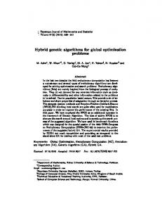
Through the plots of simulated values at their respective locations and from the reduced sample configuration points, shown in Figure 1, one may observe that the sampling schemes obtained by the optimization processes in Figure 1(e) and Figure 1(f), when compared with other, provide better coverage of the sampling points in the area. Figure 2 shows, for the simulations, the scatter plots obtained, of the order of iterations versus the mean variance of spatial prediction, by the optimization processes of SA and hybrid GA. On the plots it is observed that the optimization processes sought the lowest value for the mean variance of spatial prediction, with about 600 iterations for the simulated annealing and 50 for the hybrid GA, and the search time for the best optimized sample configuration is one hour. For the results regarding the estimates of the exponential model of semivariance function, for sampling schemes under study, shown in Table 1, we have that in all reduced samples the estimate values, on average, are very close to actual values, and the sampling grid optimized by simulated annealing showed, on average, a closer result to the value sill (C0 + C1 ), nugget (C0 ) and NE coefficient (NE = [C0 /(C0 + C1 )] × 100) of simulated data. Table 1. Estimate mean of the exponential model parameters.

Parameter Range (a) Nugget (C0 ) NE coefficient Value sill (C0 + C1 )

Ale 0.77 0.010 1.17 0.82

Sis 0.77 0.017 2.14 0.83

Pro 0.82 0.016 1.90 0.86

Fill 0.83 0.009 1.08 0.86

SA 0.82 0.006 0.72 0.87

GA 0.80 0.010 1.15 0.85

Table 2 presents the mean results related to measures regarding spatial prediction. The lowest values for the mean variance of spatial prediction σ¯02 are observed in the sampling schemes obtained by the optimization methods (SA and GA). The same results are shown in the boxplots in Figure 3(a), which highlight a low dispersion of results, especially in sampling schemes obtained by SA. When analyzing Table 2 and the boxplots from Figures 3(b) and 3(c), it appears that only the sampling schemes obtained by the GA showed values for the predict value percentage above the 75th percentile (PVPP75), closer to the actual value, with lower dispersion and lower square sum of errors (SQEPVPP75 ). Moreover, although in general the mean values

0.0

0.2

0.4

0.6

0.8

1.0 0.8 0.6 0.2

0.4

y

1.0

0.0

0.2

0.4

y

0.6

0.8

1.0

45

0.0

0.0

0.2

0.4

y

0.6

0.8

1.0

Chilean Journal of Statistics

0.0

0.2

0.4

x

0.6

0.8

1.0

0.0

0.6

0.8

1.0

0.8

1.0

0.8

1.0

1.0 0.0

0.2

0.4

y

0.6

0.8

1.0 0.8 y 0.4 0.2 0.0 0.4

0.6

(c) Pro

0.6

0.8 0.6 y 0.4 0.2 0.0

0.2

0.4 x

(b) Sis

1.0

(a) Ale

0.0

0.2

x

0.0

0.2

0.4

x

0.6

0.8

1.0

0.0

0.2

x

(d) Fill

0.4

0.6 x

(e) SA

(f) GA

Prediction variance mean 0.079 0.0815

0.086

0.078

Prediction variance mean

Figure 1. Location of the 400 sampling points (of one simulation) in the simulated area (◦) and 196 points (•).

0

400 Iterations

(a) SA

1000

0

20 Iterations

50

(b) GA

Figure 2. Scatter plots of the order of iterations versus the mean variance of the spatial prediction, of one simulation.

of the sum of predicted values above the 75th percentile (SVPP75) are different from true mean value (108.54), the lowest square sum of errors (SQESVPP75 ) are submitted by the sample configurations obtained by optimization methods (GA and GA), mainly by hybrid GA, as shown in Figures 3(d) and 3(e).

46

L.P.C. Guedes, P. J. Ribeiro Jr., S.M. De Stefano and M.A. Uribe-Opazo

Table 2. Estimate mean of measures related to spatial prediction, considering the mean value that represents the sum of simulated values of the original grid equal to 108.54.

Ale 0.091 24.61 0.15 108.50 32 × 103

Sis 0.085 24.35 0.18 104.20 43 × 103

Pro 0.092 24.56 0.26 106.40 32 × 103

Fill 0.104 25.08 0.24 109.04 60 × 103

GA 0.076 25.16 0.10 101.53 19 × 103

0.8

SA 0.078 24.41 0.23 108.20 23 × 103

SQE PVPP75

0.23

0.2

0.24

0.4

0.6

0.28

0.27 0.26

PVPP75

0.25

0.09 0.08 0.07

Prediction variance mean

0.10

0.29

Parameter σ¯02 PVPP75 SQEPVPP75 SVPP75 SQESVPP75

Ale

Sis

Fill

Pro

SA

GA

Ale

Sis

Sample Type

Ale

GA

SA

Sis

Pro

Fill

SA

GA

Sample Type

(b)

(c)

150000

SQE SVPP75

0

50

50000

100

100000

SVPP75

150

200000

200

250000

(a)

Pro Fill Sample Type

Ale

Sis

Pro

Fill

Sample Type

SA

GA

Ale

Sis

Pro Fill Sample Type

SA

GA

(d)

(e) ¯ 2 Figure 3. Boxplot of estimates: (a) variance mean of prediction (σ0 ), (b) percentage of predicted values above the 75th percentile (PVPP75), (c) squared sum of errors of the percentage of predicted values above the 75th percentile (SQEPVPP75 ), (d) sum of predicted values above the 75th percentile (SVPP75) and (e) squared sum of errors of the sum of predicted values above the 75th percentile (SQESVPP75 ).

5.

Analysis of Potassium Content Data Results

Figure 4 shows plots of potassium values in their respective locations, where the area of each point is proportional to its value for the original sample configuration (see Figure 4a) and for sampling schemes with reduced number of sample elements: simple random (see Figure 4b) regular lattice (see Figure 4c), optimized by SA (see Figure 4d) and optimized by the GA (see Figure 4e). Regularity is observed to exist in the arrangement of points on the systematic sampling and on the optimized sampling (SA and GA). In which one can identify the formation of regions with similar values and excellent coverage of the samples in the area, because there are no regions without sample points. Parameters of the exponential model of semivariance function and the mean variance of spatial prediction (σ¯02 ) are estimated for each of the reduced sampled sets and for the actual sample set, and such parameters are shown in Table 3. Comparing these results, it is noted that in all reduced samples, the values of the NE coefficient are not similar to the estimate of the initial sample. Except for the sample optimized by simulated SA, estimates with range (a) and value sill (C0 + C1 ) are similar to the value obtained in the initial sampling. It is also noted that the optimized sampling yielded a lower value for the mean variance of spatial prediction, even in relation to the value obtained by initial sampling.

47

0

0

0

40

y

y

50

50

y

80

100

100

120

Chilean Journal of Statistics

0

50

50

0

150

100

x

0

40

(b)

x

80

120

(c)

0

0

y

y

50

50

100

100

(a)

150

100

x

0

50

x

100

150

0

(d)

50

x

100

150

(e)

Figure 4. (a) Plot of potassium content values distributed on their respective locations where the area of each point is proportional to its value for the initial sample set and of samples: (b) Random simple, (c) regular lattice, (d) sampling optimized by simulated annealing algorithm and (e) sampling optimized by hybrid GA. Table 3. Estimates of semivariance function model parameters for potassium content in the samples under study and mean variance of spatial prediction.

Statistic Range (a) Nugget (C0 ) NE coefficient Value sill (C0 + C1 ) σ¯02

Initial set 56.41 0.0007 21.52 0.0034 0.0034

Ale 47.90 0.0000 0.00 0.0065 0.024

Sis 52.36 0.0006 6.96 0.0080 0.032

SA 101.35 0.0000 0.00 0.0047 0.0008

GA 45.42 0.0037 48.68 0.0076 0.0005

On the same spatial prediction grid, predicted values of reduced samples and of the initial grid are categorized, in accordance with the recommendation of the levels of potassium content for the fertilization of soybean crops in the State of Paran´ a (see Oleynik et al., 1998). Table 4 shows the amounts and percentages of predicted values, in the reduced sampling and in the initial sampling, which are in each of the intervals of classification of manure for potassium content. In general, it is observed that the sample reduced by the optimization method GA shows percentage and values of the amount of predicted values in each classification more similar to the values obtained by initial sampling. The accuracy ˆ described in Table 5, show indexes called overall accuracy (OA) and kappa statistics (K), that all sampling schemes have high accuracy, since OA ≥ 0.85 (see Anderson et al., 1976) ˆ ≥ 0.80 (see Kripendorf, 1980), and the highest values of these indexes are submitted and K by sample configuration optimized by the hybrid GA.

48

L.P.C. Guedes, P. J. Ribeiro Jr., S.M. De Stefano and M.A. Uribe-Opazo

Table 4. Estimates of number and percentage of predicted values inserted in each interval of the classification of potassium for fertilization in the State of Paran´ a (see Oleynik et al., 1998).

Statistic Number of predicted values Percentage of predicted values

Classification of Emater K ≤ 0.1 0.1 < K ≤ 0.2 0.2 < K ≤ 0.3 K > 0.3 Sum K ≤ 0.1 0.1 < K ≤ 0.2 0.2 < K ≤ 0.3 K > 0.3 Sum

Initial set 0 0 6830 10270 17100 0.00 0.00 39.94 60.06 100.00

Ale 0 0 6011 11089 17100 0.00 0.00 35.15 64.85 100.00

Sis 0 21 7555 9524 17100 0.00 0.12 44.18 55.70 100.00

SA 0 0 5541 11559 17100 0.00 0.00 32.40 67.60 100.00

GA 0 0 6916 10184 17100 0.00 0.00 40.44 59.56 100.00

Table 5. Measures of accuracy considering the variability map which is designed from the sample of 256 points, used as base map; And the variability map which is designed from the sampling configurations with 128 points, used as the reference map.

Accuracy measures Overall accuracy Kappa

Ale 0.952 0.900

Sis 0.956 0.917

SA 0.925 0.838

GA 0.995 0.900

Figure 5 shows maps of spatial variability of potassium content, taking into account the rating for fertilization in Paran´a, designed by using the grid with all data (see Figure 5a) and the reduced sampling schemes from Figure 5(b) to Figure 5(e). It is observed that the samples reduced by random simple (see Figure 5b) and optimized by simulated annealing (see Figure 5d) overestimate some regions predicted by the map of spatial variability of potassium content obtained using data of sampling that contain the entire data (see Figure 5a) not indicating the suggested classification. Variability maps which are designed through the regular lattice (see Figure 5c) and sampling scheme optimized by hybrid GA (see Figure 5e) had the highest similarity and an underestimation of some predicted regions, in relation to the variability map designed by using the grid containing all data, especially with closer approximation of each region, so understated. 6.

Conclusions

The analysis that we have been carried out for the simulations has shown that the samples obtained by the optimization methods (SA and GA), mainly by the hybrid genetic algorithm, provided estimates that were closer in similarity to the actual value, regarding the measures related to spatial prediction in non-sampled locations, and the lowest values of mean variance of spatial prediction. Give so that samples obtained by the optimization methods proved to be more reliable for spatial prediction. Analyses on reduced samples with 128 samples, for the potassium content variable, showed that the sampling optimized by the hybrid genetic algorithm had lower estimates for the mean variance of spatial prediction, even in relation to the value of this estimate obtained by means of the initial data set with 256 sampling units. In addition, in sampling optimized by hybrid genetic algorithm, estimates of the number and of the percentage of predicted values belonging to each interval of classification, used to determine the amount of product to be applied at each sampling location, were similar to the values obtained in the initial data set. These results indicate that sampling optimized by hybrid genetic algorithm, with 50% of samples, can be used in place of the sample set that contains all data in future experiments in this area, reducing half of the expenses spent with soil chemical analysis with little influence on the final results.

49

0

40

80

x

120

80 40

0

0

0

40

40

y

y

y

80

80

120

120

Chilean Journal of Statistics

40

0

120

120

0

40

x

80

120

(c)

80

y 40

0

0

40

y

80

120

(b)

120

(a)

80

x

0

40

x

80

120

0

(d)

40

x

80

120

(e)

Figure 5. Map which represents the spatial variability of K (cmolc /dm3 ) in the area, according to the classification for fertilization in soybean crops in Paran´ a, obtained from the following samplings: (a) initial set, (b) random simple, (c) regular lattice, (d) optimized by SA and (e) optimized by hybrid GA.

7.

Acknowledgements

The authors to thank to CAPES, Coordination of Improvement of Higher Education Personnel, through the Program of Social Demand and the National Council for Scientific and Technological Development (CNPq) for financial support.

References Anderson, J.F., Hardy, E.E., Roach, J.T., Witmer, R.E., 1976. A Land Use and Land Cover Classification System for use with Remote Sensor Data. Geologic Survey, Washington. Banjevic, M., Switzer, P., 2001. Optimal network designs in spatial statistics. In Royal Statistical Society Conference on Spatial Modelling, Glasgow, pp. 1-15. Boer, E.P.J., Dekkers, A.L.M., Stein, A., 2002. Optimization of a monitoring network for sulfur dioxide. Journal of Environmental Quality, 31, 121-128. Bueso, M.C., Angulo, J.M., Cruz-Sanjuli´an, J., Garc´ıa-Ar´ ostegui, J.L., 1999. Optimal spatial sampling design in a multivariate framework. Mathematical Geology, 31, 507-525. Chakrapani, Y., Rajan, K.S., 2008. Hybrid genetic-simulated annealing approach for fractal image compression. International Journal of Computational Intelligence, 4, 308-313. Costa Filho, P.A.C., Poppi, R.J., 1999. Algoritmo gen´etico em qu´ımica. Qu´ımica Nova, 27, 405-411. Couto, P., 2003. Assessing the accuracy of spatial simulation models. Ecological Modelling, 167, 181-198. Cressie, N.A.C., 1993. Statistics for Spatial Data. Wiley, New York. Diggle, P.J., Ribeiro Junior, P.J., 2007. Model-based Geostatistics. Springer, New York.

50

L.P.C. Guedes, P. J. Ribeiro Jr., S.M. De Stefano and M.A. Uribe-Opazo

Ferri, M., Piccioni, M., 1992. Optimal selection of statistical units: An approach via simulated annealing. Computational Statistics and Data Analysis, 13, 47-61. Groenigen, J.W.V., Stein, A., 1998. Constrained optimization of spatial sampling using continuous simulated annealing. Journal of Environmental Quality, 27, 1078-1086. Jackson, W.C., Norgard, J.D., 2008. A hybrid genetic algorithm with Boltzmann convergence properties. Journal of Optimization Theory and Applications, 136, 431-443. Kirpatrick, S.C., Gelatt, C. D., Vecchi, J.M.P., 1983. Optimization by simulated annealing. Science, 220, 671-680. Kriperndorf, K., 1980. Content Analysis: An Introduction to its Methodology. Sage Publications, Beverly Hills. Le, N.D., Sun, L., Zidek, J.V., 2003. Designing networks for monitoring multivariate environmental fields using data with monotone pattern. Technical report. Statistical and Aplied Mathematical Sciences Institute. Medeiros, F.L.L., Guimar˜aes, L.N.F., 2004. Hybrid genetic algorithm applied to the steady state determination problem of nonlinear dynamic systems. IEEE Computer Society Press, 1, 1-6. Miasaki, C.T., Romero, R., 2007. Um algoritmo gen´etico especializado aplicado ao planejamento da expans˜ao do sistema de transmiss˜ao com aloca¸c˜ ao de dispositivos de compensa¸c˜ao s´erie. Sba Controle e Automa¸c˜ ao, 18, 210-222. Nunes, L.M.A.F.F., Caeiro, S., Cunha, M.C., Ribeiro, L., 2005. Optimal estuarine sediment monitoring network design with simulated annealing. Journal of Environmental Management, 78, 294-304. Oleynik, J., Bragagnolo, N., Bublitz, U., Silva, J.C.C., 1998. Tabela para transforma¸c˜ ao de resultados anal´ıticos e interpreta¸c˜ ao dos resultados, Curitiba, Brazil. R Development Core Team, 2009. R: A language and environment for statistical computing. R Foundation for Statistical Computing, Vienna, Austria. Royle, J.A., 2002. Exchange algorithms for constructing large spatial designs. Journal of Statistical Planning and Inference, 100, 121-134. Ruiz-C´ardenas, R., Ferreira, M.A.R., Schmidt, A.M., 2010. Stochastic search algorithms for optimal design of monitoring networks. Environmetrics, 21, 102-112. Souza, E.G., Ribeiro, S.R.A., Uribe-Opazo, M.A., Vilas Boas, M., Silva, M.S., Johann, J.A., Molin, J.P., N´obrega, L.H.P., Oliveira, E.F., Carraro, I.A., 1999. Metodologia para an´alise da variabilidade espacial dos atributos do solo e da produtividade em uma ´area piloto de agricultura de precis˜ao. Congresso Brasileiro de Engenharia Agr´ıcola, Po¸co de Caldas, pp. 109-111. Stingel, E., 2007. Uso da geoestat´ıstica na avalia¸c˜ ao da distribui¸c˜ ao de Mahanarva fimbriolata em cana-de-a¸cu ´car. Bragantia, 66, 449-455. Wu, S., Zidek, J.V., 1992. An entropy-based analysis of data from selected NADP/NTN network sites for 1983-1986. Atmospheric Environment, 26A, 2089-2103. Zhou, Y.Y., Rao, Y.Q., Chang, C.Y., Gao, L., 2010. Hybrid genetic algorithm with simulated annealing based on best-fit strategy for rectangular packing problem. Advanced Materials Research, 379, 118-120. Zhu, Z., Stein, M.L., 2006. Spatial smapling design for prediction with estimated parameters. Journal of Agricultural, Biological and Environmental Statistics, 11, 24-44. Wollenhaupt, N.C., Wolicowski, R.P., 1994. Grid soil sampling. Better Crops with Plant Food, 78, 6-9.