Missing:
Zagazig University Faculty of Engineering Structural Engineering Department
OPTIMIZATION OF SPACE TRUSSES USING GENETIC ALGORITHM A Thesis Submitted to the Faculty of Engineering Zagazig University For The Degree of Master of Science in Structural Engineering Presented by
Eng. Osman Hamdy Osman (B. Sc., civil engineering 2009) Supervisors
Prof. Dr. Osman Shallan Head of Structural Engineering Department Zagazig University – Faculty of Engineering.
Prof. Dr. Atef Eraky Bakry
Ass. Prof. Dr. Tharwat Sakr
Prof. of Structural Engineering. Zagazig University – Faculty of Eng.
Ass. Prof., Structural Engineering Dept. Zagazig University – Faculty of Eng.
2015
First of all, I would like to introduce my greatly indebted in my work and success to ALLAH who supported me with patience and strength to complete this thesis. Cordial thanks and deep gratitude are offered to Prof. Dr. Osman Shallan, Head of Structural Engineering Department, Faculty of Engineering, Zagazig University, for his valuable guidance, encouragement and support. I would like to express my thanks and gratitude to Prof. Dr. Atef Eraky Bakry, Professor of Structural Analysis, Faculty of Engineering, Zagazig University, for suggesting the project, and for his great help, guidance, and support. Special thanks are offered to Associate Prof. Dr. Tharwat Sakr, Associate Professor, Structural Analysis, Faculty of Engineering, Zagazig University, for his guidance, support, patient and stimulating directions throughout the work also for the time he spent in refining the manuscripts and discussing the subject with me.
Osman Hamdy Osman
I
ABSTRACT Optimization of truss structures is a popular topic in structural and mechanical engineering due to their benefits to industry through the reduction of structure weight which leads to low costs and environmental friendly buildings. So optimization is important part of the design process. Size, shape and topology optimization are known categories of structural optimization aim at the selection of joint coordinates, member connectivity and element cross sections. Performing optimization for these three categories simultaneously is considered a challenge due to complexity and the restriction on the number of available cross sections used as variables. In this study, an approach for weight minimization of trusses has been developed using genetic algorithm. The proposed approach changes the design variables which constitute the Genetic Algorithm (GA) chromosome. Instead of using the nodes coordinates, member connectivity and member cross sections as design variables, it uses only free nodes coordinates and non-support nodes deflections. Topology and sizing optimization can be included using mechanical relationships based on the assumed deflections. The proposed approach was incorporated into MATLAB code to perform size, shape and
II
topology optimization simultaneously avoiding the complexity of traditional technique. Also deflection was used as design variable to avoid the restriction on available used cross sections number. Also making topology optimization using simple condition depends on the elongation of each member. Three benchmark problems were explored: size, shape, topology optimization for a10-bar plane truss, 25-bar space truss and size optimization for 72-bar space truss. The presented results produce better optimum weight than previous works in literature using less computational costs.
III
Table Of Contents ACKNOWLEDGMENTS …………………………………………………………..…………… I ABSTRACT ………………………………………………………………..…………..……..…. II TABLE OF CONTENTS ………………………………………………….……………....…….. IV LIST OF TABLES ……………………………………………………………………………….. VII LIST OF FIGURES …………………………………………………………………….….…… VIII
CHAPTER (1)
INTRODUCTION
1.1- General …………..…………………………………………………..………………..… 1 1.2- Motivation of the Study…………………………………………….……….…….……..
3
1.3- Research Objectives…………………………………………………….………….……
4
1.4- Layout of Thesis……………………………………………………………….…….…..
5
CHAPTER (2)
BACKGROUND AND LITERATURE REVIEW
2.1- General ….. ……………………………………………………………………….…….. 7 2.2- Optimization of Trusses…………………………………………………………….……. 8 2.3- Evolutionary Techniques ………………………………….…………………….………. 9 2.4- Genetic Algorithm ………………………………………………………………...……. 10 2.4.1- The GA Principle……………………………………………..…………….……. 11 2.4.1.1- Representation………………………………………………..……….. 13 2.4.1.2- Fitness Evaluation………………………………………….…………. 14 2.4.1.3- Selection………………………………………………………....……. 14 2.4.1.4- Cross-Over………………………………………………………..…… 15 2.4.1.5- Mutation………………………………………………….…......……. 16 2.4.1.6- Population Size………………………………………………..………. 17 IV
Table Of Contents 2.5- Structural Engineering Applications…………………...………………………………. 17 2.5.1- For Truss Structures………………………………………………….…...….…. 17 2.5.2- For Concrete Structures……………………….…………………....….….….…. 22 2.5.3- For Composite Structures……………………….……………….…….……..…. 23 2.5.4- Damage Detection………………………………………………………..…..…. 24
CHAPTER (3)
THE PROPOSED APPROACH
3.1- General …..…………………………………………..….………………..….………… 25 3.2- Design Variables in Traditional Technique…………………………………….……… 25 3.3- Traditional Variables Drawbacks……………………...……………………….……… 29 3.4- The proposed approach……………………………………………………..….….....… 32 3.4.1- Proposed Design Variables………………………………………………...….… 32 3.4.2- Extension to Sizing and Topology………………………………….…..…..…… 34 3.4.3- Proposed versus Traditional approaches………………….……….…..…..…….. 39 3.4.4- Handling of Constraints……………………………………………………....…....41 3.4.4.1- Constraint 1: Stability………………………………………..……....… 42 3.4.4.2- Constraint 2: Constructability………………………………....….…… 42 3.4.4.3- Constraint 3: Member stresses………………………………..…..…… 43 3.4.4.4- Constraint 4: Nodal displacements…………………………….…….… 43 3.5- The Proposed Algorithm………………………………………………………….….… 44
V
Table Of Contents CHAPTER (4)
CASE STUDY AND RESULTS
4.1- General …..……………………………………………………………………..…… 48 4.2- Benchmark Ten Bar Plane Truss ……………………………………………….…… 48 4.3- Benchmark 25-Bar Space Truss ……………………………………………..……… 58 4.3.1- Sizing Optimization of the 25-Bar Space Truss………………………..…... 58 4.3.2- Sizing, Shape and Topology Optimization of the 25-Bar Space Truss………68 4.4- Benchmark 72-Bar Space Truss ……………………………………..……………… 76
CHAPTER (5)
SUMMARY AND CONCLUSIONS
5.1- Summary …………………………….…………………………….….….….……… 92 5.2- Conclusions……………………………………………………………..…………… 92 5.3- Suggestions for Future Work………………………………………….….……….… 94
REFERENCES…………………………………………………………….………… 95
VI
List Of Tables Table Title Page (3.1) Comparison between number of bites in traditional and proposed approach………….………………………..….. 34 (4.1) Optimization results for 10-bar plan truss.……….………. 53 (4.2)
Results of previous works with same conditions..……...…
57
(4.3)
Coordinates of the joints of the 25-bar space truss...………
60
(4.4)
Group membership for 25-bar space truss....………..……
60
(4.5)
Loading conditions for 25-bar space truss……….……….
60
(4.6)
Member stresses for 25-bar space truss.……….………….
64
(4.7)
Sizing optimized 25-bar space truss results……………….
67
(4.8)
Coordinates of coordinately optimized nodes of 25-bar space truss.…………………………………………..……. Member stresses of optimized 25-bar space truss.……...…
71 72
(4.10) Size, shape and topology optimized 25-bar space truss results……………………………………………………… (4.11) Members grouping for 72-bar space truss……….……...…
75 78
(4.12) Load cases for 72-bar space truss……………….…………
78
(4.13) Members stresses for 72-bar space truss…………………..
89
(4.14) Optimization results for 72-bar space truss………………..
91
(4.9)
VII
List Of Figures Fig.
Title
(2.1)
A truss structure with its corresponding theoretical
Page
model……………………………………………………
8
(2.2)
Examples of truss optimization categories………………
9
(2.3)
Flowchart of simple GA …………………………..……
12
(2.4)
Illustration of Pareto set for a bi-objective optimization problem ………………………….…..………….………
(3.1)
10-bar plane benchmark truss.…………….……..…....…
20 28
(3.2)
Chromosome sample for 10-bar plane truss. ……………
35
(3.3)
The master flow chart of the proposed.. ……………..…
47
(4.1)
Structure of benchmark ten bar plane truss....………...…
49
(4.2)
Convergence history of benchmark ten bar plane truss structure…………………………………………………
(4.3)
51
Optimized structure of the benchmark ten bar truss for current…………………………………………………..
52
(4.4)
Load case of the ten bar truss in SAP Program (N)……..
54
(4.5)
Maximum deflection of the ten bar truss in SAP Program (mm).…………………………………………..
54
(4.6)
Optimized structure of the 10-bar truss Deb and Gulati....
55
(4.7)
Benchmark 25-bar space truss structure............................
59
(4.8)
25-bar space truss structure model in MATLAB..............
62
(4.9)
Convergence history of 25-bar space truss……...............
63
(4.10)
Load case of the 25-bar space truss in SAP program…….
65
(4.11)
Maximum deflection of the 25-bar space truss in SAP program ………………………………………………….
(4.12)
66
Shape, sizing and topology optimized 25-bar space truss structure model in MATLAB………………………...….. VIII
69
Fig.
Title
Page
(4.13)
Convergence history of 25-bar Space truss structure….…..
70
(4.14)
Load case of the 25-bar space truss in SAP program .…….
73
(4.15)
Maximum deflection of the 25-bar space truss in SAP program……………………………………………………. 73
(4.16)
Benchmark 72-bar truss structure (a) profile view, (b) element and node numbering system…………………….... 77
(4.17)
Convergence history of 72-bar space truss structure………. 80
(4.18)
Benchmark 72-bar truss structure Model in MATLAB Program.………………………………………………...…. 81
(4.19)
Load case 1 for 72-bar truss structure in ETABS program... 83
(4.20)
Maximum deflection of load case 1 for 72-bar truss structure in ETABS program………………………………. 84
(4.21)
Load case 2 for 72-bar truss structure in ETABS program... 86
(4.22)
Maximum deflection of load case 2 for 72-bar truss structure in ETABS program …………………………..….
(4.23)
87
Axial load in members due to Load Case 2 for 72-bar truss structure in ETABS program………………………………. 88
IX
Chapter (1)
Introduction
Chapter (1) INTRODUCTION 1.1 General Performing engineering design optimization, especially the optimization of complex structural systems, is an active area of research. It has become a valuable tool for engineers and designers in recent years. Although it has been applied for over fifty years, optimization in engineering has not been a commonly used design tool until high performance computing systems were made widely available. Structures are becoming lighter, stronger, and cheaper as industry adopts higher forms of optimization. This type of problem solving and product improvement is now a crucial part of the design process in today’s engineering industry. The main objective of structural optimization is saving material taking in consideration the design constrains such as allowable stresses and deflections, In other words structural optimization aims to achieve proper and optimal use of material. Saving material means saving cost and money besides also time consumed in construction process which is considered the most important factor needed to be saved in any project. Truss optimization can be classified to three categories: topology, size, and shape. All three categories generally have the 1
Chapter (1)
Introduction
objective of weight minimization without exceeding stress and displacement constraints. Topology optimization is concerned primarily with the placement of members in the truss structure relative to each other. It also deals with the number of members and the number of nodes that exist in the structure along with their support conditions [1]. Sizing optimization is concerned with the optimal selection of the cross–sectional areas of the truss members where all the nodal connectivity and the nodal locations remain fixed in the truss [1]. Shape optimization is concerned with the optimal selection of the location of the nodal points, which affect the lengths of individual members and the overall shape of the truss, which primarily refers to changing the nodal co-ordinates during optimization [1]. Genetic Algorithm (GA) is the oldest and most common form of evolutionary computation. It derives its behavior from natural evolution and genetics, following Darwin’s major principles of evolution. This method relies on random actions, and survival of the fittest to evolve solutions to optimization problems. It acquires its strength from the fact that a wide variety of problems can be driven to very good solutions by recombining parts of previous good solutions. As engineers and designers search for new optimization methods, they find that the GA can produce results never possible before.
2
Chapter (1)
Introduction
1.2 Motivation of the Study Complex structures become difficult to optimize when variable interactions increase especially when shape, size and topology optimization are made at the same time. Classical GA optimization method can produce sub-optimal results because of these interactions besides the long time consumed due to long chromosomes which depends on the number of variables and the variables space. This leads to huge number of possibilities. This may suggest that this kind of optimization should be carried out using parallel computing where the work load is divided to a group of processors. With limited computer power, the number of possibilities should be kept at a corresponding level; otherwise the calculation time will be extreme. This research is motivated by the need to reduce time consumed and complexity of making many optimization categories at the same time. GA has been shown to provide global exploration capabilities and have been used for design optimization. Many researchers worked on problems but they faced challenge in truss problems due to the existence of three categories of optimization which produce long chromosomes to describe these three categories. This leads to long execution time and complexity which direct some researchers to make optimization in two stages to overcome the complexity. Other researchers made optimization for one or two categories in the same time leading to suboptimal solution due to neglecting the third category. On the other hand the chromosome length depends on the 3
Chapter (1)
Introduction
variable limits so that some researchers tried to use low range for variables to reduce the chromosome length. For example, most of researches used low number of available cross sections to make sizing optimization.
1.3 Research Objectives The objective of this research is to develop a new approach to overcome the pre-mentioned drawbacks by using non-traditional variables. To achieve this goal new optimization strategy using GA has been developed here. It depends on using nodes coordinates and deflections as variables to make size, shape, and topology in the same time. This new technique uses only nodes coordinates and deflections as variables instead of the three traditional variables. Beside the limit of deflection variable is less than traditional cross section variable. So the chromosome which is needed in new approach is highly shorter than traditional one. And that leads to reduce the computational effort, complexity and time consumed for solution. Using deflections as design variables instead of member cross sections can lead to narrow limits of design variables and allow using any number of cross section without affecting the problem size. Also deflection is associated with nodes and cross section is associated with members. Usually the number of nodes is less than the number of members in the truss. This difference between number of members 4
Chapter (1)
Introduction
and nodes becomes high in space trusses. So using deflection as variable instead of cross section is an effective technique especially in complicated space truss where one node can connect three or four members or even more. On the other hand by looking for topology optimization (connectivity optimization), each member has two probabilities which are exist or not exist in the proposed truss. Topology optimization in this suggested strategy is not represented in the chromosome. It is derived by using a simple condition that depends on the elongation of each member which is calculated from deflections. Thus, sizing and topology
optimization
parameters
are
not
included
in
the
chromosome. They are replaced by the node deflections leading to shorter chromosome to overcome the complexity of making simultaneous sizing, topology and shape optimization.
1.4 Layout of Thesis The layout of the presented thesis is arranged as follows: Chapter one is an introduction showing the motivation of this study and its objectives. Chapter two gives a background of the structural optimization and GA method together with the required review of literature. At first, structural optimization is defined and its importance is emphasized. Literature about the optimization of trusses and GA as an evolutionary technique is then presented. Finally, different 5
Chapter (1)
Introduction
types of structural engineering applications are demonstrated. Chapter three presents the proposed technique of truss optimization using GA. It starts with design variables in traditional technique and their drawbacks followed by illustration of the proposed approach and its steps and the master flow chart of the proposed approach. Chapter four shows numerical applications of the proposed approach on three benchmark truss problems. There are 10-bar plane truss, 25-bar space truss and 72-bar space truss. It also contains comparing the results with the previous works in literature. Chapter five contains the summary of the thesis, main conclusions and the suggestion for future works in the thesis fields of interest.
6
Chapter (2)
Background and Literature
Chapter (2) BACKGROUND AND LITERATURE 2.1
General A structure in mechanics is defined by Gordon [2] as “any
assemblage of materials which is intended to sustain loads.” Optimization means making things the best. And the most proper definition of structural optimization field from economical viewpoint is making the structure weight as light as possible. The reduction of the weight of the structure obviously reduces the cost of material used leading to less total costs. Simultaneously, sustainability measures recommend the use of less material with lower embodied energy and carbon dioxide emulsion which lead to green, leadership in energy and environmental design LEED certified structures. Those points give the field of structural optimization a very high importance which necessitates being a part of design procedures. Constraints play an important role in structural optimizations such that it cannot be performed without the consideration of design constraints such as stresses, deflections and stability. Decreasing the cross sections is expected to push the structure to critical limits of stresses and deformation leading to unsafe or even unstable one. Approximately
all
engineering
optimization
problems
contain
constraints of code requirements, stress limits, serviceability conditions
7
Chapter (2)
Background and Literature
and structural rules incorporated in the optimization process using too many techniques [3].
2.2
Optimization of Trusses Truss structure is a collection of nodes (vertices) that are
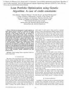
connected by a set of elements (edges) often arranged in a triangular shape. Theoretically, the bars in a truss are assumed to be connected to each other by friction-free joints. In real-life trusses though, the joints are more or less stiff due to welding or screwing the bars together. Even with some stiffness in the connections, a model with friction-free joints can accurately be used if the center of gravity axis of each bar meets in the point where the joint is exist in the model [4] as shown in figure (2.1):
Figure 2.1: A truss structure with its corresponding theoretical model [3].
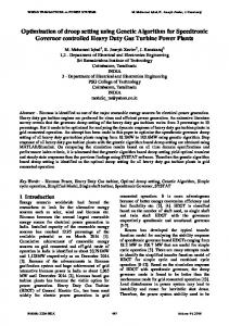
Figure (2.2) shows examples of the three types of truss optimization. The topology example shows changes in connectivity between several internal elements while the node locations remain constant. The shape optimization shows a constant topology with a variation in node locations. The size optimization shows several examples of frame element cross sectional geometries that might be
8
Chapter (2)
Background and Literature
applied to an element. Note that truss elements may only vary their cross sectional area due to the fact that this is the only property that is needed to describe the element. Topology (connectivity)
Shape
Sizing
Figure 2.2: Examples of truss optimization categories [4]
2.3 Evolutionary Techniques Particle swarm optimization (PSO) is a population-based stochastic approach for solving continuous and discrete optimization problems developed by Eberhart and Kennedy in 1995, inspired by social behavior of bird flocking or fish schooling [6]. Ant Colony Optimization (ACO) is a probabilistic technique for solving computational problems introduced by Marco Dorigo in 1992, inspired by the behavior of real ant colonies [7]. Big Bang - Big Crunch optimization (BB-BC) is a heuristic population-based
evolutionary
optimization
9
method
introduced
Chapter (2)
Background and Literature
by Osman and Eksin in 2006, inspired by the theories of the evolution of the universe [8]. Huang and Liu [6] carried out size optimization for 10- bar plane truss using particle swarm (PS). Camp [8] performed size optimization for 72-bar space truss using Big Bang – Crunch Algorithm. Li et al. [9] carried out size optimization for same truss using Heuristic Particle Swarm Optimization. Kaveh and Shojaee [7] optimized the size for the same truss using Ant Colony Optimization.
2.4 Genetic Algorithm John Holland is commonly known as the father of the GA technique. He consolidated the technique in his book Adaptation of Natural and Artificial Systems in 1975 [10, 11, and 12]. At this time though, the idea of mimicking the evolution in programming had been around for a while. In Germany, for instance, Rechenberg and Schwefel developed the evolutions strategies in the 1960s. At the same time, similar work was conducted in the USA under the name Genetic Programming. These early proposals involved mutation and selection, but not recombination, which is the key feature of GAs. Even though this new technique gave some promising results, it didn’t gain much interest at the time, probably due to the lack of computational power [12]. Over the next decade the number of scientific publications on GAs grew at approximately 40 % each year till 1995 when it peaked [13].
10
Chapter (2)
Background and Literature
The main part of these publications was different implementations of GAs. When it comes to structural optimization, Goldberg seems to be the first one to suggest the use of GAs [14, 15, and 16] in engineering design. In 1986, he used the GA technique to minimize the weight of a ten- bar aluminum plane truss and 25-bar aluminum space truss [11]. These structures are commonly used as benchmark problems in structural optimization.
2.4.1 The GA principle GAs have three characteristic operators namely, selection, crossover and mutation. In each iteration, or generation, these operators are applied on a population of possible solutions, or individuals in order to improve their fitness. Each individual is represented by a string and these strings remind very much of the natural chromosomes, leading to the name of GAs [10]. Initially, the population is created randomly, and the breeding continues until a stopping criterion is reached, e.g. the exceeding of a certain number of generations, or the absence of further improvements among the individuals. In the following sections, a more detailed review of the different GA operators is given. There are many advantages with the GA technique, primarily its simplicity and broad applicability. It can easily be modified to work on a wide range of problems [17], as contrary to
traditional
search
methods that are specified on a certain type of problem [10]. The technique is relatively robust as well; it does not tend to get stuck in
11
Chapter (2)
Background and Literature
local optimums as other techniques may do [10, 17]. Furthermore, due to the use of function evaluations rather than derivatives, it can handle discrete variables and is able to work in highly complex search spaces [17]. Figure (2.3) shows the classical flowchart for simple GA where it starts with evaluating fitness of initial population followed by the main three characteristic operators selection, cross over and mutations to produce the next generation.
Initial Population Fitness Evaluation Selection Crossover No
Mutation
Criteria Satisfied? Yes
Final Population
Figure 2.3: Flowchart of simple GA [18]
12
Chapter (2)
Background and Literature
2.4.1.1 Representation Just like the chromosome, GA string has different segments, or genes where the data are stored which are called bites and GA is only able to deal with these bites. So the variables limits numerical values should be translated to bites. That translating process called coding process. So every solution values suggested by GA will be in coded format. After that decoding process begins to translate those coded values into decimal values to calculate the fitness of suggested solutions. In the traditional GA, the string consists of a fixed-length binary string [17]. The number of genes is dependent on the number of variables that needs representation. For instance, the following string consists of five genes, g1-g5, representing five design variables:
The number of bits required in a certain gene for every design variable is calculated as [10]: 𝑁𝑜. 𝑜𝑓 𝐵𝑖𝑡𝑒𝑠 = 𝑙𝑜𝑔2 [
ximax −ximin ∆i
]
(2.1)
where ximin is the lower bound of variable i, ximax is the upper bound of variable i and ∆i is the desired precision in variable i.
13
Chapter (2)
Background and Literature
For example if the variable X has lower limit 0 and upper limit 10 with desired precision 1 so the number of bites needed to express this variable are 4 bites and the coded lower limits value will be 0000 which represents 0 where upper lower limit is 1111 which represent 10 and any binary coded string between these two strings will represent value between 0 and 10
2.4.1.2 Fitness evaluation Fitness reflects the performance of each individual so it is the measure which affects the selection of the qualified fit individuals for the next generation. In engineering optimization the fitness usually represents the objective function to be maximized or minimized and function is usually expressing the most valuable factor in the problem. For example in structure optimization problem, objective function represents the weight of structure and the goal is minimizing that weight, taking in consideration safety constrain. On the other hand if the problem is about getting the most optimized track between two points fitness will expresses the length of track. So as the track is shorter as the solution is more optimized, taking in consideration some constrains.
2.4.1.3 Selection For the reproduction, individuals with good fitness are chosen to form a mating pool. There exist many different ways to choose individuals, but the main idea is that the better the fitness is, the higher
14
Chapter (2)
Background and Literature
the probability to choose [10, 12, 17]. The mating pool has the same size as the population, but good individuals are more frequent due to duplication. A popular selection method is the tournament selection [10, 19]. In this method, small “tournaments” between randomly selected individuals are held, simply meaning that the individual with the best fitness in the group is selected. With a population size of N, N tournaments are held to fill the mating pool. This way, no copy of the worst individual is selected [19].
2.4.1.4 Cross-over With the hope of finding better solutions, the strings in the mating pool are crossed over with each other with the intention of creating a better population. Just as in the selection, there are different cross-over operators, but the main idea is that two random individuals from the mating pool are chosen as parents, and some portion of their strings are switched to create two children [10]. Three usual cross-over methods are given below [10, 17]: Single point cross-over: The two parent strings are cut at a random spot, and the pieces are put together to make two children:
Two point cross-over: The parent strings are cut twice at two random spots to create the children:
15
Chapter (2)
Background and Literature
Uniform cross-over: Each bite in the child strings are copied from either one of the parents in random process at a 50 % probability:
2.4.1.5 Mutation In the creation of new chromosome, there is always a small probability for each bit in the string to change from 0 to 1 or vice versa. If so, the child is mutated:
The purpose of this feature is to maintain the diversity amongst the individuals [10], and to prevent the algorithm from getting stuck in a local minimum [17]. The mutation probability should not be too high since in that case the GA turns into random search [17].
16
Chapter (2)
Background and Literature
2.4.1.6 Population size The size of the population should be chosen according to the complexity of the problem. In highly complex problems, the gene pool needs to be extensive enough so that the whole search space can be explored [17]. But of course, with a bigger population the computational time and effort is increased, so the upper limit of the population size should be determined by available computer power and time.
2.5 Structural Engineering applications 2.5.1 Truss Structures Rajeev and Krishnamurthy [20] and Jenkins [21] were among the first to apply GA successfully to truss sizing optimization taking in consideration stress and deflection constrains.
They applied sizing
optimization for 10-bar benchmark plane truss and for 25-bar benchmark space truss. Several researchers' in the mid-1990s tried to work on the limited topology and sizing optimization from different prospective. Hajela and Lee [22] performed topology and sizing optimization for 10 bar benchmark plane truss and for simple bridge truss type; they followed a two stage procedure. In the first stage topology optimization has been carried out for the ground structure where each nodes connected to each other nodes i.e. all possible members exist taking in consideration
17
Chapter (2)
Background and Literature
stability constrain. Many proposed topology optimized solutions for that truss are gotten from first stage. The next stage used the optimized topologies generated in the first stage as initial seeds and member-sizing optimization was performed with the consideration of stress and deflection constraints in addition to the ability of adding or removing some members in the second stage without affecting the stability of the truss. Rajan [23] performed sizing and shape optimization only and sizing with shape optimization (considering support coordinates are variable) along with limited topology optimization and taking into consideration structural constrains for 10-bar benchmark plane truss and 14-nodes plane truss. For limited topology optimization, Rajan suggested that there are some essential member for each certain problem and must exist while topology optimization is performed for non-essential members using Boolean variable 0 and 1 values where 0 means the member absence and 1 means member presence. Rajeev
and
Krishnamoorthy
[24]
presented
a
GA-based
methodology for optimal design which simultaneously considers topology, configuration, and cross-sectional parameters in a unified manner. They applied this manner on 10-bar benchmark plane truss and 18-bar plane truss. Their methodology is a two-phased approach and can handle both discrete and continuous design variables. In this procedure, they used GA to obtain appropriate lower-bound indices for each design variable in Phase 1. In Phase 2, these indices were then
18
Chapter (2)
Background and Literature
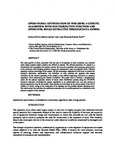
improved in an adaptive manner, in order to achieve the optimal solution. The method used a variable string length GA, which allowed variations in topology, size, and configuration. Cheng and Li [25] presented a methodology of constrained multi objective optimization problems (MOP) by integrating a Pareto GA and a fuzzy penalty function method. The Pareto GA proposed consists of the Pareto set filter and the niche as two additional operators in addition to the reproduction, crossover, and mutation to constitute five parts system. The Pareto set filter was applied to pool non-dominated points ranked 1 at each generation and drop dominated points in order to stop the loss of Pareto optimal points. Ranking was applied as a continuous labeling process such that at each generation non-dominated points (Pareto set) are selected and assigned rank 1. From the remaining population non dominated points are identified and assigned rank 2 and this process continues for rank 3, 4 and so on until the entire population is ranked. A Pareto optimal solution cannot be improved with respect to any objective without worsening at least one other objective. Points closer to Pareto optimal set is assigned higher fitness values. Any point in a pare to optimal set can become an "optimum solution" depending on the decision-makers opinion as MOP has no unique optimum that can simultaneously optimize all objectives as shown in figure (2.4).
19
Chapter (2)
Background and Literature
Figure 2.4: Illustration of Pareto set for a bi-objective optimization problem.
Niche technique prevents genetic drift and significantly distributes a population uniformly along a Pareto optimal set. In such technique an offspring replaces its parent if the offspring's fitness exceeds that of the inferior parents. This niche technique prevents the formation of a lethal and the reproduction of procedure is a steady state one. The revised penalty function method was reported to fail to work properly in a Pareto GA for constrained MOP. Thus, a fuzzy logic penalty function method is used. GA with crossover probability of 60 percent and mutation probability of 1 percent was applied. Sample cases of 4- bar pyramid truss, 72-bar space truss with two criteria (Minimum Weight and Minimum Strain energy) and four-bar truss with two criteria (Minimum weight and Minimum Deflection of two load cases). Further improvement in the field was shown by Deb and Gulati [26], in which each member’s presence or absence in the truss topology was determined by the area assigned to each member of a truss. If the
20
Chapter (2)
Background and Literature
member size was less than the predefined critical area, then the member was removed. In their research, the nodes of the trusses were divided into two categories. The first category was known as the basic nodes and then extras non-basic nodes. The presence of the basic nodes was a must to make the trusses kinematically stable. The non-basic nodes were optional. Thus, the trusses that did not have the basic nodes were excluded from further evaluation. This simultaneously size and topology optimization method was applied on 10-bar benchmark plane truss [26]. Jenkins [27] developed an idea of implementing GA without crossover. He proposed an adaptive GA that used only mutation. In his research, two kinds of mutation were used. One was the random mutation, which was similar to that used in simplified GA SGAs, in which mutation is performed with genes that are selected based on mutation probability, and the other was intelligent mutation that was performed conditionally. For instance, if the stress in a truss member exceeds the design stress then positive mutation was applied to increase the cross sectional area otherwise negative mutation is performed. Thus, this type of implementation reduced the computational expense of the method. Hultman [3] carried out size, shape and topology optimization for 10-bar benchmark plane truss using steel material while previous works used aluminum. He took into consideration allowable stress, deflection and buckling according to
Eurocode. Topology
optimization has been carried out using sizing chromosome by
21
Chapter (2)
Background and Literature
adding 50% of available sections number as zero section i.e. its cross section area is zero and whenever the members get zero sections this member will be removed so the probability to remove the member is 30%. Two runs have been carried out. The first run produced optimized size, shape and topology truss but there are some indications that the topology is suboptimal so another run has performed for the optimized one which is gotten from the first run.
2.5.2 Concrete Structures Rafiq and Southcombe [28] introduced an approach using GA to optimal design and detailing of reinforced concrete bi-axial columns. The used design variables were optimal bar size and bar detailing. The procedure attempted to keep the sectional moment capacity and cross section and get the minimum reinforcement area
leading
to
more
economical
design.
The capacity
calculation and reinforcement arrangement are made according to the British Standard (BS8110). Coello et al [29] presented a GA optimization model for the design of rectangular reinforced concrete beams subjected to a specified set of constraints. The model considered the minimization of the cost of the beam considering the costs of concrete, steel and shuttering. Simple GA was applied and results were compared to those obtained via geometric programming. Strength design procedure was adopted for which the ultimate concrete strain is 0.003 and trapezoidal stress distribution was assumed.
22
Chapter (2)
Background and Literature
The optimization of construction costs of mass concrete structures such as dams, foundation slabs, and bridge decks was carried out by Fairbairn et al. [30]. The proposed model used the GA in selecting the material type, placing temperature, height of lifts and time interval between lifts as design variables. These variables control the cost of mass concrete structures which was used as the objective function. Peng and airfield [31] presented an integrated design optimization combining the mechanism method with GAs for the optimization and design of arch bridges.
2.5.3 Composite Structures In their review of methods used to optimize composite panels, Venkataraman and Haftka [32] reported that GAs have been the most popular method for overcoming the optimization complexity of composite panels. This can be attributed to the fact that the problem is discrete in nature such that the ply orientation must be one of specific values produced by the manufacturer. Okumura et al [33] carried out Optimum design for the weaving
structure
of
three-dimensional
(3-D)
reinforced
composites. Soremekun et al [34] explored several generalized new procedures for the design of composite laminates. The problem design variables are discrete as ply angles and ply thickness can only be available in manufacturer specific values. Maximizing the buckling load of simply supported composite plate and maximizing
23
Chapter (2)
Background and Literature
the twisting displacement of cantilever composite plate was set as the two objectives of the analysis.
2.5.4 Damage detection Rao et al. [35] have proposed a method for locating and quantifying the damage in structural members using the concept of residual forces. GA has been applied for the minimization of objective function consisting of the sum squared diagonal terms of the residual force matrix. Friswell et al. [36] applied GA to eign-sensitivity analysis of damage in structures. The objective of the study was to identify the position of one or more damage sites in a structure and to estimate the extent of damage at these sites. Design variables include discrete values of damage location and continuous variable indicating the extent of damage as a percentage reduction in stiffness.
24
Chapter (3)
The Proposed Approach
Chapter (3) THE PROPOSED APPROACH 3.1 General Complex structures become difficult to optimize when variable interactions increase especially when shape, size and topology optimization are made at the same time. In this chapter, the proposed approach for GA optimization of trusses is discussed. Design variables are first introduced showing the difference between traditional variables used for combined shape, topology and size optimization and current proposed design variables. By applying the traditional design variables to applicable example, their drawbacks are illustrated. Then the proposed approach and its variables are introduced and applied to the same example illustrating the advantages of proposed approach over traditional method. Constrains are illustrated and the master algorithm and its flow chart are explained.
3.2 Design Variables in Traditional Technique In truss optimization problems, the traditional optimization variables used to represent the shape, size and topology can be listed as follows: 1-
Nodal coordinates for shape optimization containing the x, y and z coordinates of all nodes of the truss depending on the number of nodes and whether the truss is plane or space one. 25
Chapter (3)
2-
The Proposed Approach
Members cross sections for sizing optimization containing the cross section area "A" for each member of the truss depending on the number of members in the truss and the available sections for member selection.
3-
Topology matrix showing members presence for topology optimization. It contains two options one option represents the presence and other represents the absence for each member of the truss depending on the number of members in the truss. In GA, all optimization problem data are stored in the GA
chromosome leading to a chromosome length as long as the data stored in it. More data lead to more chromosome length and consequently to more time consumed and more proposed solutions for the problem. The chromosome length always depends on three parts: A- The number of optimization categories or variables which need to be optimized for the truss from the three optimization categories shape, size and topology optimization such that. Nc
L = ∑ Lc
(3.1)
c=1
where L is the total length of chromosome;
Lc
is
the
length of chromosome for category c; and Nc is the number of optimization categories applied topology and sizing, etc.).
26
(1: for sizing only, 2: for
Chapter (3)
The Proposed Approach
B- The number of objects subjected to each optimization category or variable which will be optimized, i.e. the number of members for size and topology optimization and the number of nodes for shape optimization as following equation. Lc = Nc ∗ Tc where Nc
(3.2) is the Number of objects applicable to the
optimization category (No. of members for size optimization, No. of nodes for shape optimization, etc…); and Tc is the length of chromosome per object (Number of Bits). C- The number of available profiles for each objects in the optimization category i.e. the number of available section for Size optimization or the upper, lower limits and the precision of coordinates for shape optimization as presented by following equation. ximax − ximin Tc = log 2 [ ] ∆i where ximin
(3.3)
is the lower bound of variable i; ximax
is the
upper bound of variable i; and ∆i is the desired precision in variable i. The design variable for the traditional approach is then composed of two or three coordinates for each node, cross sections and absence/presence case for each member of the whole truss. As an example, consider the 10 bar plane truss shown in figure (3.1) where nodes number 5 and 6 are coordinately variable nodes 27
Chapter (3)
The Proposed Approach
which are exposed to shape optimization while other load and support nodes are fixed and all members are exposed to sizing and topology optimization.
Figure 3.1: 10-bar plane benchmark truss.
The chromosome will consist of three parts: A-
For Shape Let the desired precision for node coordinates be 0.1 m. From truss geometric limits min. X-coordinate is 0.0 m and max. Xcoordinate is 18.28 m while min. Y-coordinate is 0.0 m and max. Y-coordinate is 9.14 m. Number of bites for X-coordinates of one node = log 2 [
18.28−0
]
0.1
= 7.51 = 8 bites. Number of bites for Y-coordinates of one node = log 2 [ 6.51 = 7 bites. 28
9.14−0 0.1
]=
Chapter (3)
B-
The Proposed Approach
For Sizing The desired precision is one section. Total number of available sections here is 226 sections used by Hultman [3]. Number of bites for size variable of one member = log 2 [
226−0 1
]
= 7.82 = 8 bites. C-
For Topology Total number of available probability is two (presence/absence) Number of bites for topology of one member = log 2 [
2−0 1
]= 1
bite. Combining Chromosome Total number of Chromosome bites = (number of bites for X coordinates + number of bites for Y-coordinates) × number of variable nodes + (No. of bites for sizing + number of bites for Topology) × Total number of truss members. Total number of Chromosome bites= (7+8)× 2+ (8+1)× 10 =120 bites.
3.3 Traditional Variables Drawbacks Traditional cross section variable depends on selecting randomly the proposed cross sections for each member from the available cross sections. The fitness value considering constrains 29
Chapter (3)
The Proposed Approach
penalty are calculated for the whole proposed truss as following equation [15, 3, 20, 7]. F(x) =
1
(3.4)
f(x)(1000v+1)
where F(x) is fitness value, 𝑓(𝑥 ) weight of truss and 𝑣 is the count of the number of constraints violated by a given solution including check of stability and constructability. So some times the individual chromosome of truss produces optimum topology, shape and member size. But due to random selection of cross sections, this combination produces section(s) smaller than minimum needed cross section(s) and this causes exceeding constrain(s) limit(s) such as stress or deflection. This unfit selected section(s) leads to unfit structure due to the penalty resulting from design violations. If these cross section(s) are increased slightly until reaching the minimum safe cross section(s), the truss will be valid and has good fitness, i.e. unsafe stress of only one member or unsafe deflection of only one node is enough to consider the whole truss unsafe. It is because of the penalty resulting from equation (3.4). In some cases individual chromosomes combination produces a good topology, shape and member size but due to random selection this combination produces section(s) larger than minimum needed cross section(s). So the outcome truss is overly weighted despite if these cross section(s) are decreased slightly until reaching the minimum safe cross section(s), then the fitness will be improved.
30
Chapter (3)
The Proposed Approach
In addition, the chromosome length needed for representing sizing variable depends on the number of discrete available cross sections equation (3.3). So if the available cross sections are few, the solution will not be accurate enough and if the available sections are many the chromosome length will be long which means more proposed solution and more time consumed. In addition, any little change in truss topology means adding or removing member(s) which leads to huge change in the proposed truss. In contrast, size and shape variables have lower and upper limits and graduated values inbetween. So it is complicated to make size, shape and topology optimization at the same time. Also making this full optimization leads to a large number of possible solutions which needs long time consumed. To overcome these drawbacks, a proposal is suggested to make topology and shape optimization only and get cross sections area from design. We have to start with suggesting that A/L = Constant value for all truss members to be able to substitute in {F}=[K]*{D} equation. After that we have to increase/decrease A/L to get the minimum safe cross sections which satisfy constrains. In that case these cross sections are not the suggested cross sections but they are final safe cross sections. However, Using cross section as a variable (traditional method) produces better result considering 'A/L' varied. This gives the opportunity to use the optimal cross sections. So new method is needed to avoid traditional drawbacks besides keeping 'A/L' varied. 31
Chapter (3)
The Proposed Approach
3.4 The proposed approach As shown the traditional method drawbacks called for the need to develop new method using new developed variables to avoid these drawbacks while keeping stiffness A/L varied between different members. The proposed idea is to use design variables only for nodes deflections and coordinates along with strain condition.
3.4.1 Proposed Design Variables The proposed approach is developed to overcome the drawbacks of using member cross sections as a variable (random case and long chromosomes). Deflection is used as a variable instead of member cross sections. While topology optimization is made by keeping members have elongation more than zero and less than allowable strain and remove the others. In other words proposed approach is using nodes deflections for non-support nodes and nodes coordinates for coordinately variable nodes as variable along with strain condition to make topology, sizing and shape optimization at the same time. This means that the design variables are now reduced to two or three coordinates for each coordinately variable node and two or three deflection components for each non-support node. Referring to the same example of the 10 -bar plane truss figure (3.1) the chromosome will consist of two parts:
32
Chapter (3)
The Proposed Approach
A- For Shape Number of bites for shape optimization is Similar to traditional case. Number of bites of X-coordinates of one node = 8 bites. Number of bites of Y-coordinates of one node = 7 bites. B- For Deflection Let the desired precision be 1 mm. Deflection variable limits range from 0.0 mm to -50.8 mm (input data of 10-bar plane truss). Number of bites for deflection variable of one node in X or Ydirection = log 2 [
0−(−50.8) 1
] = 5.66 = 6 bites.
Combining Chromosome Total number of Chromosome bites = (number of bites for Xcoordinates + number of bites for Y-coordinates) × number of variable nodes + (number of bites for deflection in X&Y direction)× Total number of non-support nodes. Total number of Chromosome bites= (7+8)× 2+ (6+6)× 4 =78 bites.
33
Chapter (3)
The Proposed Approach
Table (3.1) illustrates number of bites used in traditional and proposed methods where proposed approach uses 78 bites while Traditional one uses 120. Table 3.1: Comparison between number of bites in traditional and proposed approach Optimization Variable
Traditional Method
Shape
30
30
Size
80
ـــــــــــــــــــــ
Topology
10
ـــــــــــــــــــــ
Deflection
ــــــــــــــــــــــ
48
Total
120 Bites
78 Bites
1.32923E+36
3.02231E+23
No. of possible solutions
Proposed Method
Note: proposed approach used shape (coordinates) and deflection variables for making shape, size and topology optimization at the same time.
Also, the number of possible bites combinations, i.e. possible solutions can be calculated using equation (3.5) where two options are available for each bite. it is shown that number of possible solutions has been reduced from 1.32923E+36 to 3.02231E+23. 𝑁𝑜. 𝑜𝑓 𝑝𝑜𝑠𝑠𝑖𝑏𝑙𝑒 𝑠𝑜𝑙𝑢𝑡𝑖𝑜𝑛𝑠 = 2𝑛
(3.5)
where n is number of bites in the individual chromosomes combination.
3.4.2 Extension to Sizing and Topology Design variables of the truss in this approach are coordinates of each node (xi, yi for plane truss and xi, yi, zi for space truss, where i=1 to N, N is the number of truss coordinately variable nodes). The range of nodal coordinates are predefined or defined by the truss 34
Chapter (3)
The Proposed Approach
proposed geometric limits considering constructability constrain besides deflections of each node (ui, vi for plane truss and ui, vi, wi for space truss, where i=1 to N, N is the number of truss non-support nodes). The range of nodal deflections is defined by the code limits of allowable deflection. Figure (3.2) shows chromosome sample for the ten bars plane truss.
Figure 3.2: Chromosome sample for 10-bar plane truss.
After generating chromosome for these variables and translating these chromosomes, the proposed node coordinates for free nodes and node deflections for all non-support nodes to combine the proposed truss are obtained. Primary Topology Matrix is predefined or considered from input data which describes all logical possible distribution of members between different nodes in the truss shown in figure (3.1).
35
Chapter (3)
The Proposed Approach
Each row represents a single member. The first column represents member number from 1 to m where m is the number of truss members. Columns No. 2, 3 and 4 represent the degrees of freedom of the start node of the member and columns No. 5, 6 and 7 represent the degrees of freedom of the end node of the same member. Using
design
variables
group
which
represent
nodes
coordinates, the lengths of each member (Li) can be calculated as following: Li = √∆x 2 + ∆y 2 + ∆z 2
(3.6)
Using the other group of design variables which represent nodal deflections, the deformed length of each truss member can be calculated. The change in length (L) can be derived using the relation:
36
Chapter (3)
The Proposed Approach
ΔL = ∆x Cosθx + ∆y Cosθy + ∆z Cosθz
(3.7)
where x, y, z are the direction angles of the truss member defined by Cosθx =
x2 − x1 Li
(3.8)
Cosθy =
y2 − y1 Li
(3.9)
Cosθz =
z2 − z1 Li
(3.10)
and x, y, z are the net displacements of the member defined as: ∆x = u2 − u1
(3.11)
∆y = v2 − v1
(3.12)
∆z = w2 − w1
(3.13)
where xi, yi, zi, ui, vi, wi are the nodal coordinates and displacements of member joints, respectively. The strain of each member is then compared to the allowable strain of used material (all) as: 0.0
1e−9
(3.16)
where |K| is the determinant of stiffness matrix for the proposed truss. If the proposed truss satisfies equation (3.16), the structure is stable and the program proceeds in calculating the fitness. If equation (3.16) is not satisfied, the truss will be unstable and the proposed solution will be refused.
3.4.4.2 Constraint 2: Constructability This constrains is taken into consideration by preventing two members from having the same start and end nodes and by not allowing two or more nodes to have same coordinates. It can be achieved in 10-bar plane truss figure (3.1) by considering the proposed X-coordinates of node No. 6 larger than the proposed Xcoordinate of node No. 5. (not equal or less).
42
Chapter (3)
The Proposed Approach
3.4.4.3 Constraint 3: Member stresses Member stresses restrictions are the most important criteria in structural engineering. Member stresses must not exceed a certain limit as following. σi ≤ σall
(3.17)
where σi is the stress for member i; and σall is the allowable stress. Otherwise the truss members will fail and this means that the truss is unable to support the loads and the structure is unsafe. Stress constrains is considered in study cases of benchmark problems according to input data of each problem If the proposed truss satisfies equation (3.17), the member stresses don't violate stress constrain and the proposed truss will be accepted. Otherwise, the member stresses violate stress constrain and the proposed truss will be refused.
3.4.4.4 Constraint 4: Nodal displacements Displacement restrictions are often crucial in structural engineering. The structure is not allowed to deflect more than a certain limit as following. δi ≤ δall
(3.18)
where δi is the deflection for node i; and δall is the allowable deflection.
43
Chapter (3)
The Proposed Approach
If the proposed truss satisfies equation (3.18), the nodes deflections don't violate deflection constrain and the proposed truss will be accepted. Otherwise, the nodes deflection violate deflection constrain and the proposed truss will be refused. Stability and construability are necessary in case of making shape or/and topology optimizations. However, they are not needed in case of making only sizing optimization because in that case node coordinates and member connectivity are constant. On the contrary, stress and deflections constrains are necessary for any optimization category.
3.5
The Proposed algorithm The proposed optimization algorithm is a bit-string encoded
GA. Mutation and two point crossover type is used as reproduction operators. The master flow chart of the proposed approach is shown in figure (3.3). It starts with input data such as primary topology matrix, fixed nodes (load nodes and support nodes) coordinates, global load vector, allowable stress, allowable deflection, number of populations,
number
of
generations
and
mutation/crossover
probabilities. The next step is creating initial population according to number of population which is given in input data. Initial population is proposed values for coordinates of non-fixed nodes and deflections for non-support nodes. Each proposed solution is represented in 44
Chapter (3)
The Proposed Approach
binary coded chromosome. At this step, constructability constrain is considered by avoiding any two nodes have the same coordinates. The following process is translating this binary coded chromosome to decimal values. The proposed truss can be assembled by using these decimal values for coordinates and deflection variables. By applying strain condition, primary topology matrix will be updated to produce optimized one. So at this step, the proposed optimized truss (shape and topology) is combined. The subsequent process is making full analysis for the whole proposed optimized truss considering 'A/L=constant' to get the internal forces in each member. The next step is checking the stability for this proposal optimized truss. The proposed truss must pass stability constrain otherwise, it will be considered unfit proposed solution. The following operation is calculating proposed cross sections for truss members using design criteria equation (3.15) where these proposed cross sections is almost optimal cross sections. At this stage, the whole proposed optimized truss (shape, size and topology) is formed where this proposed truss is optimal or near optimal truss according to proposed coordinates. The next procedure is final and full analysis for this proposed optimized truss to get the member stresses and nodes deflections. At this stage, stress and deflection constrains are checked by comparing the resulted member stresses and node deflections with allowable 45
Chapter (3)
The Proposed Approach
values of stress and deflections. The truss must pass stress and deflection constrains to be valid truss otherwise, it will be unfit proposed solution. For any solution violates any constrains will take penalty to exclude this solution. On the contrary, fitness function is calculated for solution passed all constrains. Finally, if the number of generations reaches given limit the calculation processes will stop to start drawing output best truss. Otherwise, new generation will deformed using cross over and mutations probabilities.
46
Chapter (3)
The Proposed Approach Input data
Create initial population Input data For Each chromosome
Create initial population Assemble the basic structure and translate the For Each chromosome binary chromosome in to FEM structure
Update Assemble the basic topology structure matrix and translate the binary chromosome in to FEM structure Analyze the truss suggesting A/L=Const. Update topology matrix Check on the stability Analyze the truss and get cross sections No
Passed and stability Check on constructability Yes No
Calculate the suggested sections
Passed Yes
Calculate Elementthe Stresses and Node Deflection Calculate suggested sections Penalty any violations Calculate Element Stresses and Node Deflection
Evaluate Fitness Penalty anythe violations Reached
Termination Evaluate the Fitness Criteria Not Reached
Reached
Termination Cross over & Mutation Criteria Not Cross over & Mutation Selection & New Generation Reached
Translate the binary chromosome and draw the truss and results
Figure
Translate the binary chromosome andThe drawmaster the truss and results 3.3: flow chart
approach 47
of the proposed.
Chapter (4)
Case Study And Results
Chapter (4) CASE STUDY AND RESULTS 4.1 General Structure optimization is very important in structural design process especially in truss design. It aims to produce the most optimum safe truss with minimum weight. In this chapter, the proposed approach is applied to benchmark problems to evaluate its capabilities through comparison with studies conducted in the literature. The first problem is size shape and topology optimization for benchmark ten bar plane truss which is commonly used to verify new truss optimization approach. The second optimized size benchmark 25-bar space truss and extended to size shape and topology optimization for the same truss. The third problem is size optimization for benchmark 72-bar space truss.
4.2 Benchmark Ten bar Plane Truss The first problem is shape, sizing and topology optimization for ten bar plane truss. This ten-bar truss is often used as a benchmark problem in structural optimization. This structure is frequently found in literature related to plane truss optimization [3, 5]. The truss has two vertical supports with distance 'a' of 9.144 meters (360 inches) and two loads 'F'of 445.374 KN (100 kips) at 9.144 and 18.288 meters from the lower support as shown in figure (4.1). Aluminum is used, with Modulus of elasticity E equals 68.95 GPa (104 ksi), density ρ equals 2, 768 kg/m3 (0.1 lb/in3) and element stresses are 48
Chapter (4)
Case Study And Results
limited to 172.37 MPa (25 ksi) in both tension and compression while buckling and own weight are ignored. The displacements are limited to 50.8 mm (2 in) both horizontally and vertically. Shape is optimized for coordinates of nodes P1 and P3 only within geometry limits of the truss while support and load nodes are fixed.
Figure 4.1: Structure of benchmark ten bar plane truss.
These input data and constrains are similar to those used in previous works for ten bar plane truss to make fair comparison between this study and previous works. The problem was solved using GA by Rajeev [20], Coello [15], Galante [37], Ruiyi, GuiLiangjin, Zijie [38], Schmid [39], Rajan [23], Hajela and Lee [22], Xu [40], Rajeev [24], Wenyan [41], Rahami [42] and Gulati [26]. It was also solved by Baugh Jr. et al. [43] using hybrid search method. Moreover, it was solved by Liu et al. [6] using particle swarm. 49
Chapter (4)
Case Study And Results
Using the suggested technique, weight is minimized utilizing GA with parameters as following: Population size is 600 which it is sufficient to show the capability of the proposed approach for this example, maximum generation 200 which it is enough to obtain best fitness for this population size, crossover probability equals 0.9 and mutation probability equals 0.05. Available cross sections are similar to cross sections (226 cross sections) were used by Hultman [3]. As mentioned earlier, number of available cross section doesn't affect chromosome length or GA efficiency. As illustrated in chapter 3, 226 cross sections were used for making full optimization for 10-bar plane truss. It consumed 120 bites using traditional while 78 bites only were consumed using current approach Figure (4.2) shows the convergence history of the ten bars plane truss example. The mean fitness value is plotted against the generation number to clarify how the GA converges to the optimum solution. Two population sizes were used. These are 400 and 600 where 400 produced truss weighs 4824 lb. while 600 produced truss weighs 4762.1 lb. Using population size more than 600, there is not reduction in truss weight. As depicted from the figure, the fitness value (which reflects the truss weight taking into consideration violated constrains ) improvement is very limited during the first 30 generation, and then greatly improved till the 100th generation after which stability is observed. 50
Chapter (4)
Case Study And Results
Figure 4.2: Convergence history of benchmark ten bar plane truss structure.
Figure (4.3) shows the shape of optimized truss. This optimized topology is similar to that resulted in all researches which made topology along with shape optimization.
51
Chapter (4)
Case Study And Results
Figure 4.3: Optimized structure of the benchmark ten bar truss for current. study.
Nodal coordinates for coordinately variable node P3 is (11.73, 6.4) while node P1 is deleted. Table (4.1) shows member cross section areas and their stresses. Maximum stress absolute value for our resulted optimized truss is 161.50 MPa in member M1 which represents 93.7% of allowable stress. And the maximum deflection absolute value investigated in the optimum solution is 50.763 mm for node P2 in Y direction which reaches 99.92% of the maximum permissible value which means that the selected cross sections are almost optimized.
52
Chapter (4)
Case Study And Results
Table 4.1: Optimization results for 10-bar plan truss.
Box section Element
dimensions, (mm)
Cross section
Stress,
% of allowable
area, (cm2)
(MPa)
stress
M1
200x200x5
39.00
161.5
93.70%
M2
400x400x10
156.00
-57.9
33.60%
M3
260x260x12.5
123.74
-39.9
23.10%
M4
180x180x12
80.65
-56.8
32.90%
M5
350x350x10
136.00
46.97
27.20%
M6
400x400x12
186.26
49.12
28.50%
Verification of the proposed procedure was carried out using SAP2000 program to double check for the deflection. This was conducted because this example is controlled by deflection; i.e. deflection has reached allowable value (99.92%) before stress reached its allowable value. The applied loads of the final optimized truss are shown in figure (4.4) while the maximum nodal displacement is shown in figure (4.5). The maximum actual deflection absolute value as shown is 50.796 mm while our MATLAB code produced 50.763 mm for node P2 in Y direction which is approximately matched.
53
Chapter (4)
Case Study And Results
Figure 4.4: Load case of the ten bar truss in SAP Program (N).
Figure 4.5: Maximum deflection of the ten bar truss in SAP Program (mm). (N,mm). 54
Chapter (4)
Case Study And Results
Table (4.2) lists the results encountered in literature for the 10 member benchmark problem compared with the results of the proposed approach of the present study. The results shows that the current proposed approach resulted in the most optimized value of fitness (weight) which is less than all results found in the literature except those obtained by Deb and Gulati [26] where they obtained a better solution (4731.65 lb.) when the constructability condition wasn't considered. Figure (4.6) shows their optimum solution which contains two duplicated members. One member was between nodes P6 & P4 and the other member was between nodes P6 & P2. This is considered undesirable overlap and unpractical to implement [26].
Figure 4.6: Optimized structure of the 10-bar truss Deb and Gulati [15] (4731.65 Lb).
When they considered constructability condition, i.e. preventing members overlapping, they obtained a truss weight of (4899.15 lb.) and produced same topology produced in the current study. Most of literature studies considered limited optimization categories i.e. shape and sizing or topology and sizing or only size 55
Chapter (4)
Case Study And Results
optimization. That is to avoid the complexity resulted from making full optimization (size, shape, and topology at the same time). Rajeev [24] made size, shape and topology optimization at the same time, but used limited topology optimization and conducted the analysis using two stages as mentioned earlier in Chapter 2. This is different from the current approach which considers size, shape and topology optimization at the same time, through one stage and without any limitation on topology optimization. Schmid [39] made size and shape optimization for topology optimized truss (6-bar truss) as shown in figure (4.3).
56
Chapter (4)
Case Study And Results
Table 4.2: Results of previous works with same conditions. Optimization Search
Weight
category
Method
(lbs.) Size
Shape
Topology
Rajeev (1992)
LINRM
√
6249.00
Rajeev (1992)
SUMT
√
5932.00
Rajeev (1992)
GRP-UI
√
5727.00
Rajeev (1992)
M-5
√
5725.00
Rajeev (1992)
M-3
√
5719.00
Genetic algorithm
√
5613.84
Coello (1994)
Genetic algorithm
√
5586.59
Rajeev (1992)
CONMIN
√
5563.00
Rajeev (1992)
OPTDYN
√
5472.00
Galante (1996)
Genetic algorithm
√
Xu (2010)
Genetic algorithm
√
5078.23
Kripakaran et al. (2007)
Hybrid method.
√
5073.03
Li et al. (2006)
Particle swarm
√
5060.9
Su Ruiyi et al. (2009)
Genetic algorithm
√
Schmid (1997)
Genetic algorithm
√
Rajan (1995)
Genetic algorithm
√
√
4962.1
Hajela (1995)
Genetic algorithm
√
√
4942.7
Rajeev (1997)
Genetic algorithm
√
√
4925.80
Wenyan (2005)
Genetic algorithm
√
√
4921.25
Rahami (2008)
Genetic algorithm
√
√
4855.2
Rajeev (1992)
√
5119.3
√ √
√
Note
4962.07 4962.10
Two stages
Const. Genetic algorithm
√
√
4731.65
constrain not considered
Gulati (2001) Const. Genetic algorithm
√
√
4899.15
constrain considered
Current study (2015)
Genetic algorithm
√
57
√
√
4762.1
Chapter (4)
Case Study And Results
4.3 Benchmark 25-Bar Space Truss The second benchmark problem is 25-bar space truss optimization. This structure is frequently found in the literature related to space truss optimization [44]. Most of the works found in the literature are related to sizing optimization for which node location and connectivity are already known. In current work, at first sizing optimization was applied to compare with the results of previous works. Then the full optimization procedure was applied to obtain the most optimum shape, topology and sections. This simultaneous optimization for 25-bar space truss has also been conducted by Wenyan [41] and Rahami [42] where shape optimization was made for nodes number 3, 4, 5, 6, 7, 8, 9 and 10 as shown in figure (4.7).
4.3.1. Sizing optimization of the 25-bar space truss Figure (4.7) shows the truss shape. The coordinates of joints, the member groups for section selection and applied loads are shown in tables (4.3), (4.4) and (4.5) respectively. Aluminum is used with modulus of elasticity E equals 68.95 GPa (104 ksi) and density, ρ equals 2,768 kg/m3 (0.1lb. /in3) and element stresses are limited to 275.8 MPa (40 ksi) in both tension and compression while buckling and own weight are ignored. The displacements of nodes are limited to 8.9 mm (0.35 in) in all directions.
58
Chapter (4)
Case Study And Results
Figure 4.7: Benchmark 25-bar space truss structure (inch=2.54 cm).
59
Chapter (4)
Case Study And Results
Table 4.3: Coordinates of the joints of the 25-bar space truss.
Node 1 2 3 4 5 6 7 8 9 10
X (m) -0.9525 0.9525 -0.9525 0.9525 0.9525 -0.9525 -2.54 2.54 2.54 -2.54
Y (m) 0 (Inch) 0 0.9525 0.9525 -0.9525 -0.9525 2.54 2.54 -2.54 -2.54
Z (m) 5.08 (Inch) 5.08 2.54 2.54 2.54 2.54 0 0 0 0
Table 4.4: Group membership for 25-bar space truss.
Group Number 1 2 3 4 5 6 7 8
Members 1-2 1-4, 2-3, 1-5, 2-6 2-5, 2-4, 1-3, 1-6 3-6, 4-5 3-4, 5-6 3-10, 6-7, 4-9, 5-8 3-8, 4-7, 6-9, 5-10 3-7, 4-8, 5-9, 6-10
Table 4.5: Loading conditions for 25-bar space truss. Node
Fx (KN)
Fy (KN)
Fz (KN)
1
4.45374
-44.5374
-44.5374
2
0
-44.5374
-44.5374
3
2.22687
0
0
6
2.672244
0
0
These similar to data input and constrains are used in previous works.
60
Chapter (4)
Case Study And Results
The problem was solved using GA by Rajeev [20], Zhu [45], Erbatur et al. [46], Coello et al. [47], Cao [48], Togan [49], Tayfun [44], Wu [50], Wenyan [41] and Rahami [42]. It was solved by Talaslioglu [51] using Bi population-Based GA with enhanced interval search. It was also solved by Li et al. [9] using heuristic particle swarm optimization. It was solved by Lee et al. [52] using Harmony Search Heuristic Algorithm. It was also solved by Camp [8] using Bang –Crunch Algorithm. It was also solved by Kaveh and Shojaee [7] using Ant Colony Optimization. All these pre-mentioned researches made sizing optimization only for 25-bar space truss. The set of available cross section areas for this problem is A=i*0.64516 (cm2) where i ranges from 1 to 50. Using this technique weight is minimized by GA with parameters as following: Population size is 400 where it is the minimum adequate value to show the capability of the proposed approach for this example, maximum generation 100 where it is enough to reach best fitness for this population size, crossover probability equals 0.9 and Mutation probability equals 0.05. Figure (4.8) shows the model of 25-bar space truss in MATLAB while Figure (4.9) shows the convergence history of the 25-bar space truss example. The fitness mean value is plotted against the generation number to clarify how the GA converges to the optimum solution. As obvious from the plot, the fitness value is greatly improved from first generation till the 60th generation after which stability is observed. 61
Chapter (4)
Case Study And Results
Figure 4.8: 25-bar space truss structure model in MATLAB.
62
Chapter (4)
Case Study And Results
Figure 4.9: Convergence history of 25-bar space truss. structure.
Table (4.6) shows the resulted member cross section areas and their stresses where maximum absolute stress value is 124.17 MPa (18.01 ksi) in member 6-3 which represents 45.02% of allowable stress. Moreover, maximum absolute deflection value in the optimum solution is 8.89 mm for node 1 in Y direction which reaches 99.89% of the maximum permissible value meaning that the selected cross sections are almost economic.
63
Chapter (4)
Case Study And Results
Table 4.6: Member stresses for 25-bar space truss.
Member
Area (cm2)
Length (m)
Weight (kg)
Axial Force (KN)
Abs. stress value (MPa)
1-2
0.65
1.91
0.34
-0.03
0.48
2-6
1.94
3.31
1.78
16.97
87.68
1-5
1.94
3.31
1.78
13.88
71.71
2-3
1.94
3.31
1.78
3.15
16.29
1-4
1.94
3.31
1.78
4.51
23.30
1-6
23.23
2.71
17.44
248.06
106.80
1-3
23.23
2.71
17.44
45.53
19.60
2-5
23.23
2.71
17.44
204.28
87.95
2-4
23.23
2.71
17.44
66.87
28.79
6-5
10.97
1.91
5.78
-29.94
27.30
3-4
10.97
1.91
5.78
13.85
12.63
5-4
0.65
1.91
0.34
-5.44
84.25
6-3
0.65
1.91
0.34
-8.01
124.17
4-9
5.16
4.60
6.57
3.31
6.40
5-8
5.16
4.60
6.57
-14.70
28.48
6-7
5.16
4.60
6.57
-20.53
39.78
3-10
5.16
4.60
6.57
6.01
11.63
6-9
2.58
4.60
3.29
-10.27
39.78
5-10
2.58
4.60
3.29
-7.35
28.48
4-7
2.58
4.60
3.29
1.65
6.41
3-8
2.58
4.60
3.29
3.00
11.63
5-9
23.23
3.39
21.79
-89.77
38.65
6-10
23.23
3.39
21.79
-125.40
53.99
4-8
23.23
3.39
21.79
20.19
8.69
3-7
23.23
3.39
21.79
36.67
15.79
216.061
Max. stress
124.174
Weight (kg)
64
Chapter (4)
Case Study And Results
Verification of the proposed procedure was carried out using SAP2000 program to check the deflection since this example is controlled by deflection. Figure (4.10) shows the load case and figure (4.11) shows the maximum absolute deflection value which is 8.8002 mm while MATLAB produced 8.89 mm for node 1 in Y direction which is approximately matched.
Figure 4.10: Load case of the 25-bar space truss in SAP program (KN).
65
Chapter (4)
Case Study And Results
Figure 4.11: Maximum deflection of the 25-bar space truss in SAP program (mm).
Table (4.7) lists the results encountered in the literature for only sizing optimized 25 member space truss problem compared with the results of the proposed approach. As shown in the results, the proposed approach resulted in the most optimized value of fitness (weight) which is less than all results found in literature. the sizing optimized truss weight is 476.33 lb. where it represents 98.54% of the best result encountered in the literature (Togan [49]).
66
67
1.8
2.3
0.2
0.1
0.8
1.8
3
546.01
A2
A3
A4
A5
A6
A7
A8
Weight (lbs.)
562.93
2.6
2.1
0.8
0.1
0.1
2.6
1.9
0.1
1986
493.8
3.4
0.4
0.9
0.1
0.1
3.2
1.2
0.1
2000
[46]
493.94
3.4
0.5
1.1
1.4
0.1
3.2
0.7
0.1
1994
[47]
485.05
3.4
0.5
0.9
1.9
0.1
3.4
0.5
0.1
1996
483.35
3.4
0.5
1
2
0.1
3.4
0.3
0.1
2008
[49]
485.9
3.4
0.7
1
1.9
0.1
3.4
0.1
0.1
2009
BGAwEIS
[51]
484.85
3.4
0.5
1
2.1
0.1
3.4
0.3
0.1
2009
HPSO
[9]
Talaslioglu Li et al.
484.85
3.4
0.5
1
2.1
0.1
3.4
0.3
0.1
HSH 2005
[52]
al.
Lee et
484.85
3.4
0.5
1
2.1
0.1
3.4
0.3
0.1
2007
BB-BC
[8]
Camp
484.85
3.4
0.5
1
2.1
0.1
3.4
0.3
0.1
2007
[7] ACO
Kaveh
484.85
3.4
0.5
1
2.1
0.1
3.4
0.3
0.1
2011
[44]
Tayfun
Interval Search.
Optimization, HSH: Harmony Search Heuristic Algorithm, BGAwEIS: Bi population-Based Genetic Algorithm with Enhanced
BB-BC: Big Bang –Crunch Algorithm, Algorithm, ACO: Ant Colony Optimization, HPSO: Heuristic Particle Swarm
0.1
1992
[20]
A1
(area in2)
Design variable Rajeev
Zhu [45] Erbatur Coello Cao [48] Togan
Table 4.7: Sizing optimized 25-bar space truss results.
476.33
3.6
0.4
0.8
1.7
0.1
3.6
0.3
0.1
2015
study
Current
Chapter (4) Case Study And Results
Chapter (4)
Case Study And Results
4.3.2. Sizing, shape and topology optimization of the 25-bar space truss. To perform full optimization of the same problem, using the size, shape and topology where optimized simultaneously using the same data input, constrains, and GA parameters. For shape optimization case, the coordinates limits for coordinately variable node number 4 in X-direction From 20 to 60 inch and in Y-direction from 40 to 80 inch and in Z-direction from 90 to 130 inch where another variable nodes 3,5 and 6 are considered symmetric to node number 4. Moreover, for support node number 8, in X-direction from 40 to 80 inch; and in Y-direction from 100 to 140 in other support nodes number 7, 9 and 10 are considered symmetric to node number 8. Figure (4.12) shows the resulted topology, sizing and shape optimized 25-bar space truss in MATLAB. It is worthwhile to note that 6 members are removed (Groups number 1, 4, 5 and one member from group number 2). Figure (4.13) shows the convergence history of the 25 bars space truss example, where the mean fitness value is plotted against the generation number. It is clear that the fitness value greatly improves from the first generation up to the 40th generation after which stability is observed. By comparing with convergence history of only sizing optimization case, it is shown that the optimum solution is reached more early in case of simultaneous sizing, shape and topology optimization. This is due to the fact that using node coordinates along with its 68
Chapter (4)
Case Study And Results
deflections allows changing in member length and its elongation and leads to more options in topology optimization which allows removing unnecessary members.
Figure 4.12: Shape, sizing and topology optimized 25-bar space truss structure model in MATLAB.
69
Chapter (4)
Case Study And Results
Figure 4.13: Convergence history of 25-bar Space truss structure.
Table (4.8) shows the coordinates of coordinately variable nodes number 3, 4, 5 and 6 along with coordinates of support nodes number 7, 8, 9 and 10. It is shown that the truss turned into wideness in Y-direction.
70
Chapter (4)
Case Study And Results
Table 4.8: Coordinates of coordinately optimized nodes of 25-bar space truss.
Node
X (m)
Y (m)
Z (m)
3
-1.0312
1.4834
3.1445
4
1.0312
1.4834
3.1445
5
1.0312
-1.4834
3.1445
6
-1.0312
-1.4834
3.1445
7
-1.4275
3.5357
0.00
8
1.4275
3.5357
0.00
9
1.4275
-3.5357
0.00
10
-1.4275
-3.5357
0.00
Table (4.9) shows the resulted member sections and their stresses where maximum absolute stress value is 119.62 MPa (17.35 ksi) in member 2-5 which represents 43.73% of allowable stress and maximum absolute deflection value is 8.8975 mm for node 1 in the Y direction which reaches 99.97% of the maximum permissible value which means that the selected cross sections are almost economic.
71
Chapter (4)
Case Study And Results
Table 4.9: Member stresses of optimized 25-bar space truss. . Membe r 1-2 2-6
Area (cm2)
Length (m)
Weight Axial Force (kg) (KN) Removed 0.56 3.76
Abs. stress value (MPa)
0.65
3.14
1-5
0.65
3.14
0.56
6.89
106.82
2-3 1-4 1-6
0.65
3.14
0.56
3.33
51.61
5.81
2.44
3.92
53.99
92.98
1-3
5.81
2.44
3.92
33.98
58.52
2-5
5.81
2.44
3.92
69.47
119.62
2-4 6-5 3-4 5-4 6-3 4-9
5.81
2.44
3.92
28.18
48.53
0.65
5.94
1.06
1.56
24.22
5-8
0.65
5.94
1.06
0.32
5.01
6-7
0.65
5.94
1.06
0.86
13.34
3-10
0.65
5.94
1.06
1.77
27.50
6-9
0.65
4.49
0.80
1.14
17.64
5-10
0.65
4.49
0.80
0.43
6.63
4-7
0.65
4.49
0.80
2.07
32.04
3-8
0.65
4.49
0.80
2.35
36.38
5-9
6.45
3.78
6.74
5.08
7.87
6-10
6.45
3.78
6.74
13.53
20.97
4-8
6.45
3.78
6.74
24.57
38.09
3-7
6.45
3.78
6.74
27.90
43.24
51.79
Max Stress
119.62
58.21
Removed
Removed Removed Removed Removed
Weight (kg)
Verification of the proposed procedure was carried out using SAP2000 program to check the deflection since this example is controlled by deflection. Figure (4.14) shows the load case and figure (4.15) shows the maximum absolute deflection absolute value which is 8.8889 mm while MATLAB produced 8.8975 mm for node 1 in Y direction which is approximately matched. 72
Chapter (4)
Case Study And Results
Figure 4.14: Load case of the 25-bar space truss in SAP program (KN).
Figure 4.15: Maximum deflection of the 25-bar space truss in SAP program (mm).
73
Chapter (4)
Case Study And Results
Table (4.10) shows the literature results compared with the proposed approach result. As seen from the table, the current proposed approach resulted in the most optimized value of fitness (weight) which is less than all results found in literature. For sizing, shape and topology optimized truss the weight is 114.171 lb. where it represents 99.83% of the best result encountered in the literature (Rahami [42]). As shown in table (4.10), Wenyan [41], Rahami [42] and current study removed member groups number 1, 4 and 5. But the current study removed one extra member from group number 2 while the other members in the same group are remained. It proves the capability of making topology optimization using strain condition along with deflections and coordinates variable. Also it shows the sensitivity of this method for removing all members which can be removed. The weight of sizing optimized 25-bar space truss using current method is 476.33 lb, while it is 114.171 lb using same method for optimizing size, shape and topology of the same truss. The reduction in weight (76.03% reduction) shows the importance of making full (size, shape and topology) optimization for trusses.
74
Chapter (4)
Case Study And Results
Table 4.10: Size, shape and topology optimized 25-bar space truss results.
Wu [50] Members and its groups
1-2 2-6 1-5 2-3 1-4 1-6 1-3 2-5 2-4 6-5 3-4 5-4 6-3 4-9 5-8 6-7 3-10 6-9 5-10 4-7 3-8 5-9 6-10 4-8 3-7
Group 1
Group 2
Group 3
Group 4 Group 5
Group 6
Group 7
Group 8
X4 (in) Y4 (in) Z4 (in) X8 (in) Y8 (in) Weight (lb.)
1995 0.1 0.2 0.2 0.2 0.2 1.1 1.1 1.1 1.1 0.2 0.2 0.3 0.3 0.10 0.10 0.10 0.10 0.2 0.2 0.2 0.2 0.90 0.90 0.90 0.90 41.07 53.47 124.6 50.8 131.48 136.2
Wenyan Rahami Current study [41] [42] 2005 2008 2015 2 Cross section area (in ) Removed Removed Removed 0.10 0.10 0.10 0.10 0.10 0.10 0.10 0.10 0.10 0.10 0.10 Removed 0.90 0.90 0.90 0.90 0.90 0.90 0.90 0.90 0.90 0.90 0.90 0.90 Removed Removed Removed Removed Removed Removed Removed Removed Removed Removed Removed Removed 0.10 0.10 0.10 0.10 0.10 0.10 0.10 0.10 0.10 0.10 0.10 0.10 0.10 0.10 0.10 0.10 0.10 0.10 0.10 0.10 0.10 0.10 0.10 0.10 1.00 1.00 1.00 1.00 1.00 1.00 1.00 1.00 1.00 1.00 1.00 1.00 39.91 38.7913 40.60 61.99 66.111 58.40 118.23 112.9787 123.80 53.13 48.7924 56.20 138.49 138.891 139.20 114.74 114.3701 114.171
75
Chapter (4)
Case Study And Results
4.4 Benchmark 72-Bar Space Truss The third problem is size optimization for 72-bar space truss. This truss consists of 4 support nodes and four symmetric levels. Each level has 4 free nodes and 18 members as shown in figure (4.16). This structure is frequently found in literature related to space truss optimization [44]. Allowable stress equals 172.37 MPa (25 ksi) for all members from 1 to 72 in both tension and compression while buckling and own weight are ignored. Allowable displacement equals 6.35 mm (0.25 in) in only X and Y directions for only nodes numbers 17, 18, 19 and 20. Modulus of elasticity E equals 68.95 GPa (104 ksi) and Density of material equals 2, 768 kg/m3 (0.1 lb. /in3). Members grouping are shown in table (4.11). These input data and constrains are similar to those used in previous works for 72-bar space truss to make fair comparison between this study and previous works. Two load cases are considered as shown in table (4.12). In the first load case, the truss is controlled by deflection constrain where in the second one, the truss is controlled by stress constrain.
76
Chapter (4)
Case Study And Results
Figure 4.16: Benchmark 72-bar truss structure (a) profile view, (b) element and node numbering system.
77
Chapter (4)
Case Study And Results
Table 4.11: Members grouping for 72-bar space truss.
Group No.
Group Members
Group No.
Group Members
A1
1,2,3,4
A9
37,38,39,40
A2
5,6,7,8,9,10,11,12
A10
41,42,43,44,45,46,47,48
A3
13,14,15,16
A11
49,50,51,52
A4
17,18
A12
53,54
A5
19,20,21,22
A13
55,56,57,58
A6
23,24,25,26,27,28,29,30
A14
59,60,61,62,63,64,65,66
A7
31,32,33,34
A15
67,68,69,70
A8
35,36
A16
71,72
Table 4.12: Load cases for 72-bar space truss. Load Case
Node
Fx (KN)
Fy (KN)
Fz (KN)
1
17
22.24
22.24
-22.24
17
0.00
0.00
-22.24
18
0.00
0.00
-22.24
19
0.00
0.00
-22.24
20
0.00
0.00
-22.24
2
The problem was solved using GA by Adeli and Kamal [53], Cao [48], Venkayya [54], Schmit and Farshi [55], Khan et al. [56], Erbatur et al. [46], Gellatly and Berke [57], Barbaso and Lemonge [58] Ayvaz and Aydın [59], Dede et al. [60] and Tayfun [44]. It was also solved by Talaslioglu [51] using BipopulationBased GA with enhanced interval search. It was solved also by Camp [8] using Big Bang-Crunch Algorithm; and was solved by
78
Chapter (4)
Case Study And Results
Perez and Behdinan [61] using Particle Swarm Optimization Algorithm. Cross section variable is continuous as it is used in most of literature studies. Continues variable in traditional method has upper and lower limits besides precision for the graduated values inbetween these limits as it shown in equation (3.3). These limits and precision values affect chromosome length which represents the variable. But in current study, continuous cross section means cross sections which are obtained directly from design equation (3.15). So the current approach doesn't need limits or precision while the equation produces cross sections have infinite accuracy without any increment in chromosome length. Using this technique weight is minimized by GA with parameters as following: Population size is 800 where it is the minimum adequate value to show the capability of the proposed approach for this example; maximum generation 200 where it is enough to reach best fitness for this population size, crossover probability equals 0.9 and mutation probability equals 0.05. Two deflection variables are used for each node one is for load case 1 and the other is for load case 2. Table (4.13) shows the stresses in each member of 72-bar truss for both load cases. Figure (4.17) shows the convergence history of the 72 bars space truss
79
Chapter (4)
Case Study And Results
example. The mean fitness value is plotted against the generation number to clarify how the GA converges to the optimum solution. As investigated from the plot, the fitness value is greatly improved from first generation till the 150th generation after which stability is observed. Figure (4.18) shows the 72-bar space truss model in MATLAB program.
Figure 4.17: Convergence history of 72-bar space truss structure.
80
Chapter (4)
Case Study And Results
Figure 4.18: Benchmark 72-bar truss structure Model in MATLAB Program.
81
Chapter (4)
Case Study And Results
For load case 1 Maximum absolute stress value is 111.6 MPa (16.186 ksi) for member 55 which represents 64.74% of allowable stress. Maximum absolute deflection value investigated in the optimum solution is 6.34492 mm for node 17 in X and Y direction which represents 99.95 % of allowable deflection. Verification of the proposed procedure was carried out for load case 1 using ETABS program to check deflection since this load case is controlled by deflection. Figure (4.19) shows the load case and figure (4.20) shows the maximum absolute deflection value which is 6.3 mm while MATLAB produced 6.34492 mm for node 17 in X and Y direction which is approximately matched.
82
Chapter (4)
Case Study And Results
Figure 4.19: Load case 1 for 72-bar truss structure in ETABS program (N).
83
Chapter (4)
Case Study And Results
Figure 4.20: Maximum deflection of load case 1 for 72-bar truss structure in ETABS program (mm).
For load case 2 Members 55, 56, 57 and 58 got maximum stress value 167.40 MPa (24.28 ksi) which represents 97.144% of allowable stress. While nodes 17, 18, 19 and 20 got maximum deflection value 0.99949 mm in X and Y directions which represents 15.74 % of allowable deflection. Using ETABS program, a verification of the proposed procedure was carried out for load case 2 to check deflection and stress since this load case is controlled by stress. Figure (4.21) shows 84
Chapter (4)
Case Study And Results
the load case and figure (4.22) shows the maximum absolute deflection value which is 1 mm while MATLAB produced 0.99949 mm for nodes 17, 18, 19 and 20 in X and Y directions which is approximately matched. Figure (4.23) shows axial load in Load Case 2 where axial force in members 55, 56, 57 and 58 is 4.206 kip and its stress equals 167.34 MPa (24.27 ksi) where it was 24.28 from MATLAB which is approximately matched. As shown in table (4.13), the truss in load case (1) is controlled by deflection constrain while it is controlled by stress constrain in load case (2). So it is not possible to optimize topology for that truss considering these two load cases. Table (4.14) lists the results encountered in literature for the 72 member space truss problem compared with the results of the proposed approach. As illustrated from the results, the current proposed approach resulted in the most optimized value of fitness (weight) which is less than all results found in literature. Current study resulted size optimized truss weighs 375.77 lb, which represents 99.06% of the best result recorded in the literature Adeli [53].
85
Chapter (4)
Case Study And Results
Figure 4.21: Load case 2 for 72-bar truss structure in ETABS program (N).
86
Chapter (4)
Case Study And Results
Figure 4.22: Maximum deflection of load case 2 for 72-bar truss structure in ETABS program (mm).
87
Chapter (4)
Case Study And Results
Figure 4.23: Axial load in members due to Load Case 2 for 72-bar truss structure in ETABS program (kip).
88
Chapter (4)
Case Study And Results
Table 4.13: Members stresses for 72-bar space truss.
Member No.
Cross section group
Cross section Area (cm2)
1 2 3 4 5 6 7 8 9 10 11 12 13 14 15 16 17 18 19 20 21 22 23 24 25 26 27 28 29 30 31 32 33 34 35 36
A1 A1 A1 A1 A2 A2 A2 A2 A2 A2 A2 A2 A3 A3 A3 A3 A4 A4 A5 A5 A5 A5 A6 A6 A6 A6 A6 A6 A6 A6 A7 A7 A7 A7 A8 A8
12.865 12.865 12.865 12.865 3.717 3.717 3.717 3.717 3.717 3.717 3.717 3.717 0.434 0.434 0.434 0.434 0.143 0.143 10.268 10.268 10.268 10.268 3.572 3.572 3.572 3.572 3.572 3.572 3.572 3.572 0.193 0.193 0.193 0.193 0.232 0.232
Length (m)
Weight (kg)
152.40 152.40 152.40 152.40 340.77 340.77 340.77 340.77 340.77 340.77 340.77 340.77 304.80 304.80 304.80 304.80 431.06 431.06 152.40 152.40 152.40 152.40 340.77 340.77 340.77 340.77 340.77 340.77 340.77 340.77 304.80 304.80 304.80 304.80 431.06 431.06
5.42 5.42 5.42 5.42 3.51 3.51 3.51 3.51 3.51 3.51 3.51 3.51 0.37 0.37 0.37 0.37 0.17 0.17 4.33 4.33 4.33 4.33 3.37 3.37 3.37 3.37 3.37 3.37 3.37 3.37 0.16 0.16 0.16 0.16 0.28 0.28
89
Load Case 1 (Abs. value) Axial Stresses Forces (MPa) (KN)
23.09 7.47 31.09 7.47 7.96 5.96 4.85 6.05 6.05 4.85 7.96 5.96 0.18 0.18 0.18 0.18 0.13 0.04 12.54 5.47 22.24 5.47 5.83 8.27 5.74 5.03 5.03 5.74 5.83 8.27 0.27 0.09 0.09 0.27 0.22 0.40
17.94 5.81 24.17 5.81 21.42 16.04 13.04 16.28 16.28 13.04 21.42 16.04 4.10 4.10 4.10 4.10 9.31 3.10 12.22 5.33 21.66 5.33 16.32 23.17 16.07 14.07 14.07 16.07 16.32 23.17 13.83 4.61 4.61 13.83 9.59 17.27
Load Case 2 (Abs. value) Axial Stresses Forces (MPa) (KN)
22.55 22.55 22.55 22.55 0.36 0.36 0.36 0.36 0.36 0.36 0.36 0.36 0.49 0.49 0.49 0.49 0.18 0.18 21.31 21.31 21.31 21.31 1.02 1.02 1.02 1.02 1.02 1.02 1.02 1.02 0.13 0.13 0.13 0.13 0.18 0.18
17.53 17.53 17.53 17.53 0.96 0.96 0.96 0.96 0.96 0.96 0.96 0.96 11.26 11.26 11.26 11.26 12.41 12.41 20.75 20.75 20.75 20.75 2.86 2.86 2.86 2.86 2.86 2.86 2.86 2.86 6.91 6.91 6.91 6.91 7.68 7.68
Chapter (4)
Case Study And Results
Table 4.13: Members stresses for 72-bar space truss (continued).
Member No.
Cross section group
Cross section Area (cm2)
37 38 39 40 41 42 43 44 45 46 47 48 49 50 51 52 53 54 55 56 57 58 59 60 61 62 63 64 65 66 67 68 69 70 71 72
A9 A9 A9 A9 A10 A10 A10 A10 A10 A10 A10 A10 A11 A11 A11 A11 A12 A12 A13 A13 A13 A13 A14 A14 A14 A14 A14 A14 A14 A14 A15 A15 A15 A15 A16 A16
4.540 4.540 4.540 4.540 2.948 2.948 2.948 2.948 2.948 2.948 2.948 2.948 0.220 0.220 0.220 0.220 0.413 0.413 1.118 1.118 1.118 1.118 3.160 3.160 3.160 3.160 3.160 3.160 3.160 3.160 2.499 2.499 2.499 2.499 3.186 3.186
Total Weight (kg)
Length (m)
Weight (kg)
152.40 152.40 152.40 152.40 340.77 340.77 340.77 340.77 340.77 340.77 340.77 340.77 304.80 304.80 304.80 304.80 431.06 431.06 152.40 152.40 152.40 152.40 340.77 340.77 340.77 340.77 340.77 340.77 340.77 340.77 304.80 304.80 304.80 304.80 431.06 431.06
1.91 1.91 1.91 1.91 2.78 2.78 2.78 2.78 2.78 2.78 2.78 2.78 0.19 0.19 0.19 0.19 0.49 0.49 0.47 0.47 0.47 0.47 2.98 2.98 2.98 2.98 2.98 2.98 2.98 2.98 2.11 2.11 2.11 2.11 3.80 3.80 170.46
90
Load Case 1 (Abs. value) Axial Stresses Forces (MPa) (KN)
Load Case 2 (Abs. value) Axial Stresses Forces (MPa) (KN)
2.80 4.72 12.14 4.72 8.90 5.69 4.72 5.56 5.56 4.72 8.90 5.69 0.71 0.00 0.00 0.71 1.60 0.27 12.50 0.27 3.87 0.27 5.12 10.90 4.31 4.54 4.54 4.31 5.12 10.90 6.54 2.09 2.09 6.54 2.76 8.41 Max. Stress
23.44 23.44 23.44 23.44 1.33 1.33 1.33 1.33 1.33 1.33 1.33 1.33 0.98 0.98 0.98 0.98 1.87 1.87 18.73 18.73 18.73 18.73 3.91 3.91 3.91 3.91 3.91 3.91 3.91 3.91 1.87 1.87 1.87 1.87 2.36 2.36 Max. Stress
6.17 10.39 26.75 10.39 30.18 19.32 16.00 18.86 18.86 16.00 30.18 19.32 32.36 0.00 0.00 32.36 38.73 6.46 111.60 2.39 34.61 2.39 16.19 34.49 13.65 14.36 14.36 13.65 16.19 34.49 26.17 8.37 8.37 26.17 8.66 26.39 111.60
51.64 51.64 51.64 51.64 4.53 4.53 4.53 4.53 4.53 4.53 4.53 4.53 44.49 44.49 44.49 44.49 45.19 45.19 167.42 167.42 167.42 167.42 12.39 12.39 12.39 12.39 12.39 12.39 12.39 12.39 7.48 7.48 7.48 7.48 7.40 7.40 167.42
0.4791
0.1
0.1
0.1579
0.5501
0.3449
0.4984
379.31
A11
A12
A13
A14
A15
A16
Wight (Lbs.)
0.1
A7
A10
0.5689
A6
0.5137
1.1567
A5
A9
0.1
A4
0.1
0.1
A3
A8
0.5332
A2
91
380.32
0.6749
0.3981
0.5501
0.1557
0.1049
0.1
0.5227
0.5177
0.1
0.1
0.5028
1.283
0.1
0.1
0.4933
1.8562
1996
1986
2.0259
Cao [48]
Adeli [53]
A1
Design variable area (in2)
381.2
0.506
0.377
0.557
0.161
0.1
0.1
0.532
0.611
0.1
0.1
0.524
1.246
0.1
0.1
0.524
1.818
1971
Venkayya [54]
388.63
0.608
0.341
0.594
0.158
0.151
0.1
0.548
0.264
0.1
0.1
0.579
1.107
0.1
0.1
0.503
2.078
1974
Schmit [55]
387.67
0.5317
0.4378
0.5614
0.1519
0.1583
0.1
0.5273
0.5814
0.1
0.1
0.5244
1.2526
0.1
0.1
0.5259
1.8589
1979
383.12
0.103
0.122
0.525
1.91
0.103
0.11
0.498
1.31
0.111
0.103
0.535
0.535
0.521
0.379
0.544
0.161
2000
Khan et al Erbatur [56] et al. [26]
395.97
0.342
0.453
0.773
0.149
0.1
0.1
0.608
0.552
0.1
0.1
0.542
1.024
0.1
0.1
0.521
1.464
1971
Gellatly [57]
Table 4.14: Optimization results for 72-bar space truss.
384.1341
0.1
0.1
0.462033
1.862385
0.100075
0.102094
0.483267
1.315822
0.102617
0.1
0.573289
0.654788
0.726192
0.293503
0.577252
0.15346
2003
Barbaso [58]
406.03
0.508
0.35
0.587
0.174
0.174
0.174
0.477
0.508
0.174
0.174
0.587
0.978
0.174
0.174
0.587
2.046
2000
407.37
0.431
0.431
0.587
0.174
0.22
0.22
0.508
0.431
0.287
0.174
0.508
1.457
0.174
0.174
0.477
2.046
2003
Ayvaz Dede et al. [59] Disc. [60] Disc.
380.783
0.1
0.1
0.513
1.86
0.105
0.101
0.523
1.25
0.1
0.1
0.53
0.62
0.51
0.37
0.555
0.156
2009
379.85
0.5922
0.3922
0.5507
0.1565
0.1005
0.1004
0.5172
0.5209
0.1012
0.1
0.5269
1.2476
0.1
0.1
0.5059
1.8577
2007
381.91
0.1
0.1
0.5185
1.7427
0.1
0.1
0.5193
1.3079
0.1095
0.1
0.5464
0.5142
0.5619
0.4967
0.5092
0.1615
2007
Talaslioglu Camp [8] Perez [51] BB-BC [59] PSO BGAwEIS
382.35
0.604
0.442
0.604
0.154
0.118
0.109
0.55
0.505
0.1
0.1
0.469
1.288
0.1
0.1
0.496
1.702
2011
Tayfun [44]
375.77
0.49385
0.38727
0.48978
0.1733
0.064083
0.034095
0.45689
0.70363
0.03593
0.029919
0.5536
1.5916
0.022226
0.06734
0.57611
1.9941
2015
Current study
Chapter (4) Case Study And Results
Chapter (5)
Summary And Conclusions
Chapter (5) SUMMARY AND CONCLUSIONS 5.1 Summary When dealing with simultaneous size, shape and topology optimization of trusses, the number of possible solutions reaches great levels, which need long chromosome and long calculation time. In this thesis, an approach is proposed for optimization of plane and space trusses using GA method where GA design variables are changed to contain node deflections instead of member sections and connectivity in addition to nodal coordinates. The proposed procedure was applied to three of the classical truss benchmark problems to carry out sizing, topology and shape optimization and the results are investigated and compared with that found in previous works.
5.2 Conclusions Based on the conducted study, the following conclusions can be drawn:
92
Chapter (5)
1-
Summary And Conclusions
GA is considered a suitable tool for truss optimization with different categories and configurations.
2-
The proposed approach for selecting the design variables succeeded to reduce the chromosome length needed to represent truss variables that lead to reduction in number of possible solutions and the calculation time and effort by using a few numbers of chromosomes.
3-
As the truss cross sections are not included in the design variables, it is possible in the proposed approach to choose sections from huge numbers of a predetermined set without any increase in the chromosome length. The results were compared to the results of previous work found in literature where the presented results produce better optimum weight than previous results.
4-
As compared with literature, more optimized solutions are obtained
by
using
the
proposed
approach
with
less
computational costs. The number of bites used and number of possible solutions required to solve the problem is significantly reduced.
93
Chapter (5)
5-
Summary And Conclusions
The results obtained utilizing the proposed approach are more optimized when compared with previous research. Less weight was obtained for all studied benchmarks for combined optimization or even sizing optimization.
6-
The proposed GA technique allows full optimization (size, shape and topology) in the same time without increase in the consumed time.
7-
The proposed approach proved that GA still has the flexibility as a tool for structural optimization.
5.3 Suggestions for Future Work Based on the work in the present thesis and the results obtained, the following may be valid points for future research: 1.
To use more revolutionary techniques as the real coded GA, Particle Swarm optimization (PSO), Ant Colony optimization (ACO) and Big Bang - Big Crunch optimization (BB-BC).
2.
To apply these methods to more advanced structural types such as tensigrity structures.
94
References
REFERENCES [1]
Soumya, S. P. (2006) “Investigation Of Genetic Algorithm Design Representation For Multi-Objective Truss Optimization." Office of graduate studies of Texas - A&M University.
[2]
Gordon, J. G. (1978) “Structures Or Why Things Don’T Fall Down." Penguin, Baltimore.
[3]
Hultman, M. (2010) “Weight Optimization Of Steel Trusses By A Genetic Algorithm." Institude of technology, Lund university.
[4]
Heyden, S. Dahlbom, O. Olsson, A. Sandberg, G. (2005) “Introduktion Till Introduktion Till Strukturmekaniken." Institude of technology, Lund university.
[5]
Brian, J. A. (2005) “Size And Shape Optimization Of Frame And Truss Structures Through Evolutionary Methods." College of graduate studies, IDAHO university.
[6]
Lijuan, Li. Huang, Z. Liu, F. (2006) “An Improved Particle Swarm Optimizer For Truss Structure Optimization." International Conference on Computational Intelligence and Security. Volume 1.Pages 924-928.
[7]
Kaveh, A. Shojaee, S. (2007) “Optimal Design Of Skeletal Structures Using Ant Colony Optimization." International Journal of Numerical Methods in Engineering, Volume 70, Issue 5, pages 563–581.
[8]
Camp, C.V. (2007) “Design Of Space Trusses Using Big Bang-Big Crunch Optimization." journal of Structural Engineering, Volume 133, Issue 7 , pages 999–1008.
[9]
Li, L.J. Huang, Z.B. Liu, F. (2009) “A Heuristic Particle Swarm Optimization Method Fortruss Structures With Discrete Variables." Computers & Structures, Volume 87, Issues 7–8,Pages 435–443.
[10] Kalyanmoy, D. (1997) “Genetic Algorithm In Search And Optimization." International Workshop on Soft Computing and Intelligent Systems. Pages 58-87.
95
References [11] Goldberg, D. E. (1989) “Genetic Algorithms In Search, Optimization And Machine Learning." New York: Addison-Wesley. [12] Reeves, C. R. Jonathan, E. (2002) “Genetic Algorithms: Principles And Perspectives – A Guide To Ga Theory." New York: Springer US. [13] Alander, J. T. (1999) “An Indexed Bibliography Of Genetic Algorithm Implementations. Bibliography." University of Vaasa Department of Information Technology and Production Economics. [14] Coello Coello, C. A. Christiansen, A. D. (2000) “Multiobjective Optimization Of Trusses Using Genetic Algorithms." Computers and Structures. Volume 75, issue 6. Pages 647- 660. [15] Coello Coello, C. A. Rudnik, M. Christiansen, A. D. (1994) “Using Genetic Algorithms For Optimal Design Of Trusses." The Sixth International Conference on Tools with Artificial Intelligence. Pages 8894. [16] Kaveh, A. Kalatjari, V (2004) “Size/Geometry Optimization Of Trusses By The Force Method And Genetic Algorithm." ZAMM – Zeitschrift für Angewandte Mathematik und Mechanik. Volume 84, issue 5. Pages 347-357. [17] Sivanandam S. N. Deepa S. N. Algorithms." Berlin: Springer.
(2008) “Introduction To Genetic
[19] Rothlauf, F. (2006) “Representations For Genetic And Evolutionary Algorithms." Berlin: Springer. [20] Rajeev, S. Krishnamoorthy, C.S. (1992) “Discrete Optimization Of Structures Using Genetic Algorithms." Journal of Structural Engineering, Volume 118, Issue 5, Pages 1233–1250. [21]
Jenkins, W. (1992) “Plane Frame Optimum Design Environment Based on Genetic Algorithm." Journal of structural engineering, volume 118, Issue 11, Pages 3103-3112.
[22] Hajela, P. Lee, E. (1995) “Genetic Algorithms In Truss Topological Optimization." International Journal of Solids and Structures. Volume 32, issue 22. Pages 3341-3357.
96
References [23] Rajan, S.D. (1995) “Sizing, Shape And Topology Design Optimization Of Trusses Using Genetic Algorithm." Journal of Structural Engineering Volume 121, Issue 10, Pages 1480–1487. [24]
Rajeev, S. Krishnamoorthy, CS. (1997) “Genetic Algorithms-Based Methodologies For Design Optimization Of Trusses." Journal of Structural Engineering, Volume 123, Issue 3, Pages 350–358.
[25]
Cheng, F. and Li, D. (1997). ”Multiobjective Optimization Design with Pareto Genetic Algorithm.” Journal of structural engineering, volume 123, Issue 9, Pages 1252-1261.
[26] Deb, K. Gulati, S (2001) “Design Of Truss-Structures For Minimum Weight Using Genetic Algorithms." Finite elements in analysis and design Volume 37, Pages 447-465. [27]
Jenkins, W. (2002) “A decimal-coded evolutionary algorithm for constrained optimization." Journal of computer and structure, volume 80, Issue 5-6, Pages 471-480.
[28]
Rafiq, M. Southcombe, C. (1998) “Genetic algorithms in optimal design and detailing of reinforced concrete biaxial columns supported by a declarative approach for capacity checking." Journal of computer and structure, volume 69, Issue 4, Pages 443-457.
[29]
Coello, C. C., Carlos, A., and Christiansen, A. D. (1997), "A Simple Genetic Algorithm for the Design of Reinforced Concrete Beams", Engineering with Computers, Springer-Verlag, Volume 13, No. 4, Pages 185-196, 1997.
[30]
Fairbairn, E. M. R., Silvoso, M. M., Filho, R. D. T., Alves, J. L. D., and Ebecken, N. F. F. (2004), " Optimization of Mass Concrete Construction Using Genetic Algorithms", Computers and Structures, Volume82, Pages 281-299.
[31]
Peng, D. M. airfield, C.A. (1999), "Optimal Design of Arch Bridges by Integrating Genetic Algorithms and the Mechanism Method", Engineering Structures, Volume 21, Pages.75–82.
97
References [32]
Venkataraman, S. Haftka, R. T. (1999), "Optimization of Composite Panels "A Review", Proceedings of the 14th Annual Technical Conference of the American Society of Composites, Dayton, OH.
[33]
Okumura, T. Yokoyama, A. NagaiS, K. Maekawa, Z. (1995), "Optimum Design Of Weaving Structure Of 3-D Woven Fabric Composites By Using Genetic Algorithms", Composite Structures, Volume 32, Pages 417-426.
[34]
Soremekun, G. Gurdal, Z. Haftka, R. T. Watson, L.T. (2001), "Composite Laminate Design Optimization by Genetic Algorithm with Generalized Elitist Selection", Computers and Structures, Volume 79, Pages 131-143.
[35]
Rao, M. A., Srinivas, J. Murthy, B. S. N. (2004), "Damage Detection in Vibrating Bodies Using Genetic Algorithm", Computers and Structures, Volume82, Pages 963-968.
[36]
Friswell, M. I., Penny, J. E. T., and Garvey, S. D. (1998), "A Combined Genetic `and Eign-sensitivity Algoritm for the Location of Damage in Structures", Journal of Computers & Structures, Volume 69, Pages 443-457.
[37] Miguel G. (1996) “Genetic Algorithms As An Approach To Optimize Real-World Trusses." International journal for Numerical Methods in engineering. Volume 39, issue 3. Pages 361-382. [38] Su Ruiyi, G. F (2009) “Truss Topology Optimization Using Genetic Algorithm With Individual Identification Technique." The World Congress on Engineering 2009 Volume II. [39] Schmid, L. (1993) “Discussion Of 'Discrete Optimization Using Genetic Algorithms." Journal of Structural Engineering, Vol. 118, Issue. 5, Pages 1233-1250. [40] Xu, T. Zuo, W.Z. Xu, T. Song, G. Li, R. (2010) “An Adaptive Reanalysis Method For Genetic Algorithm With Application To Fast Truss Optimization." Acta Mechanica Sinica, Volume 26, Issue 2, Pages 225-234.
98
References [41] Tang, W. Tong, L. Gu, Y. (2005) “Improved Genetic Algorithm For Design Optimization Of Truss Structures With Sizing, Shape And Topology Variables. " International Journal for Numerical Methods in Engineering, Volume 62, Issue 13, pages 1737–1762. [42] Rahami, H. Kaveh, A. Gholipour, Y. (2008) “Sizing, Geometry And Topology Optimization Of Trusses Via Force Method And Genetic Algorithm." Engineering Structures, Volume 30, Issue 9, Pages 2360– 2369. [43] Prakash, K. Abhinav, G. Baugh, Jr. John, W. (2007) “A Novel Optimization Approach For Minimum Cost Design Of Trusses." Computers & Structures. Volume 85, issue 23-24. Pages 1782-1794. [44] Dede, T. Ayvaz S.Y. (2011) “Weight Minimization Of Trusses With Genetic Algorithm." Applied Soft Computing, Volume 11, Issue 2, Pages 2565–2575.
[45] Zhu, D.M. (1986) “An Improved Templeman’S Algorithm For Optimum Design Of Trusses With Discrete Member Size." Engineering Optimization, Volume 9, Issue 4, pages 303-312. [46] Erbatur, F. Hasancebi, O. Tutuncu, I. Kılıc, H. (2000) “Optimal Design Of Planar And Space Structures With Genetic Algorithm." Computers & Structures, Volume 75, Issue 2, Pages 209–224. [47] Coello, C.A.C. Rudnick, M. Christiansen, A.D. (1994) “Using Genetic Algorithm For Optimal Design Of Trusses." IEEE, Pages 88– 94. [48] Cao, G. (1996) “Optimized Design Of Framed Structures Using A Genetic Algorithm." The University of Memphis. [49] Togan, V. Daloglu, A.T. (2008) “An Improved Genetic Algorithm With Initial Population Strategy And Self-Adaptive Member Groupings." Computers & Structures, Volume 86, Issues 11–12,Pages 1204–1218. [50]
Wu S-J, Chow P-T. (1995) “Integrated Discrete And Configuration Optimization Of Trusses Using Genetic Algorithms." Computers & Structures, Volume 55, Issue 4, Pages 695–702.
99
References [51] Talaslioglu, T. (2009) “A New Genetic Algorithm Methodology For Design Optimization Of Truss Structures: Bi Population-Based Genetic Algorithm With Enhanced Interval Search. " Modelling and Simulation in Engineering, Volume 2009 , Article ID 615162, 28 pages. [52] Lee, K.S. Geem, Z.W. Lee, S.H. Bae, K.W. (2005) “The Harmony Search Heuristic Algorithm For Discrete Structural Optimization," Engineering Optimization, Volume 37, Issue 7,pages 663-684. [53]
Adeli, H. Kamal, O. (1986) “Efficient Optimization Of Space Trusses." Computers & Structures, Volume 24, Issue 3, Pages 501–511.
[54] Venkayya, V.B. (1971) “Design Of Optimum Structures." Computers & Structures, Volume 1, Issues 1–2, Pages 265–309. [55] Schmit, L.A. Farshi, B. (1974) “Some Approximation Concepts For Structural Synthesis. " The American Institute of Aeronautics and Astronautics (AIAA) Journal, Vol. 12, Issue 2, Pages 692-699. [56] Khan, M.R. Willmert, K.D. Thornton, W.A. (1979) “An Optimality Criterion Method For Large-Scale Structures." The American Institute of Aeronautics and Astronautics (AIAA) Journal, Vol. 17, Issue 7, Pages 753-761. [57]
Gellaty, R.A. Berke, L. (1971) “Optimal Structural Design." Technical report AFFDL-TR-70- 165, Air Norce Flight Dynamics Laboratory, Wright–Patterson Air force Base,Ohio.
[58] Barbaso, H.J.C. Lemonge, A.C.C (2003) “A New Adaptive Penalty Scheme For Genetic Algorithms." Information Sciences, Volume 156 Issue 3-4, Pages 215 - 251. [59] Ayvaz, Y. Aydın. Z. (2000) “Optimum Design Of Trusses Using A Genetic Algorithm," The Second International Conference on Engineering Using Metaphors from Nature, Pages. 159–168. [60] Dede, T. Ayvaz, Y. Bekiroglu, S. (2003) “Optimization Of Truss Structures Using Value Encoding In A Genetic Algorithm." The Seventh International Conference on the Application of Artificial Intelligence to Civil and Structural Engineering, paper 38. [61] Perez, R.E. Behdinan, K. (2007) “Particle Swarm Approach For Structural Design Optimization." Computers & Structures, Volume 85, Issues 19–20, Pages 1579–1588.
100
ﺟﺎﻣﻌـــــــــﺔ اﻟﺰﻗﺎزﯾﻖ ﻛﻠﯿــــﺔ اﻟﮭﻨﺪﺳــــــــــﺔ ﻗﺴﻢ اﻟﮭﻨﺪﺳﺔ اﻹ ﻧﺸﺎﺋﯿﺔ
أﻣﺜﻠﯿﺔ اﻟﺠﻤﺎﻟﻮﻧﺎت اﻟﻔﺮاﻏﯿﺔ ﺑﺎﺳﺘﺨﺪام اﻟﺨﻮارزﻣﺎت اﻟﻮراﺛﯿﺔ رﺳﺎﻟﺔ ﻣﻘﺪﻣﺔ ﻣﻦ
اﻟﻤﮭﻨﺪس /ﻋﺜﻤﺎن ﺣﻤﺪى ﻋﺜﻤﺎن ﻟﻨﯿﻞ درﺟﺔ اﻟﻤﺎﺟﺴﺘﯿﺮ ﻓﻰ اﻟﻌﻠﻮم اﻟﮭﻨﺪﺳﯿﮫ ﻓﻲ اﻟﮭﻨﺪﺳﺔ اﻻﻧﺸﺎﺋﯿﺔ ﺗﺤﺖ إﺷــﺮاف
أ.د /ﻋﺜﻤﺎن ﺷﻌﻼن أﺳﺘﺎذ اﻹﻧﺸﺎءات -و رﺋﯿﺲ ﻗﺴﻢ اﻟﮭﻨﺪﺳﺔ اﻹﻧﺸﺎﺋﯿﺔ ﻛﻠﯿﺔ اﻟﮭﻨﺪﺳﺔ -ﺟﺎﻣﻌﺔ اﻟﺰﻗﺎزﯾﻖ
أ.د.م /ﺛﺮوت ﺻﻘﺮ
أ .د /ﻋﺎطـــﻒ ﻋﺮاﻗﻲ ﺑﻜﺮى
أﺳﺘﺎذ ﻣﺴﺎﻋﺪ ﺑﻘﺴﻢ اﻟﮭﻨﺪﺳﺔ اﻹﻧﺸﺎﺋﯿﺔ ﻛﻠﯿﺔ اﻟﮭﻨﺪﺳـــــﺔ -ﺟﺎﻣﻌﺔ اﻟﺰﻗﺎزﯾﻖ
أﺳﺘﺎذ اﻹﻧﺸﺎءات -ﻗﺴﻢ اﻟﮭﻨﺪﺳﺔ اﻹﻧﺸﺎﺋﯿﺔ ﻛﻠﯿﺔ اﻟﮭﻨﺪﺳـــــــﺔ -ﺟﺎﻣﻌﺔ اﻟﺰﻗﺎزﯾﻖ
٢٠١٥
ﻣﻠﺨﺺ اﻟﺮﺳﺎﻟﺔ ﯾﻤﻜﻦ ﺗﻄﻮﯾﺮ ﻋﻤﻠﯿﺔ أﻣﺜﻠﯿﺔ اﻟﺠﻤﺎﻟﻮﻧﺎت وﺗﻼﻓﻰ ﻋﯿﻮب اﻟﻄﺮق اﻟﺘﻘﻠﯿﺪﯾﺔ ﻷﻣﺜﻠﯿﺔ اﻟﺠﻤﺎﻟﻮﻧﺎت ﺑﺎﻻﺿﺎﻓﺔ اﻟﻰ ﺗﻘﻠﯿﻞ اﻟﻌﻤﻠﯿﺎت اﻟﺤﺴﺎﺑﯿﺔ اﻟﻤﺴﺘﺨﺪﻣﺔ وﺑﺎﻟﺘﺎﻟﻰ اﻟﻮﻗﺖ اﻟﻤﺴﺘﮭﻠﻚ ﻟﮭﺬه اﻟﺤﺴﺎﺑﺎت ﻣﻊ اﻟﺤﺼﻮل اﯾﻀﺎ ﻋﻠﻰ ﻧﺘﺎﺋﺞ اﻓﻀﻞ ﻣﻦ ﻧﺘﺎﺋﺞ اﻻﺑﺤﺎث اﻟﺴﺎﺑﻘﺔ ﻋﻦ طﺮﯾﻖ اﺳﺘﺨﺪام اﻧﻮاع ﺟﺪﯾﺪه ﻣﻦ اﻟﻤﺘﻐﯿﺮات ﻏﯿﺮ اﻟﺘﻰ ﺗﺴﺘﺨﺪم ﺑﺎﻟﻄﺮق اﻟﺘﻘﻠﯿﺪﯾﺔ ﺣﯿﺚ ﺗﻢ اﺳﺘﺒﺪال اﻟﻤﺘﻐﯿﺮات اﻟﺨﺎﺻﺔ ﺑﻘﻄﺎﻋﺎت اﻟﻌﻨﺎﺻﺮ اﻟﻤﺨﺘﻠﻔﺔ وﺣﺎﻻت ﺗﻮزﯾﻊ اﻟﻌﻨﺎﺻﺮ ﺑﯿﻦ اﻟﻨﻘﺎط اﻟﻤﺨﺘﻠﻔﺔ ﺑﻤﺘﻐﯿﺮ ﺧﺎص ﺑﺎزاﺣﺔ اﻟﻨﻘﺎط اﻟﺮﺋﯿﺴﯿﺔ دون ﻧﻘﺎط اﻟﺪﻋﺎﺋﻢ ﺑﺎﻻﺿﺎﻓﺔ اﻟﻰ اﺳﺘﺨﺪام ﻣﺘﻐﯿﺮ اﺣﺪاﺛﯿﺎت اﻟﻨﻘﺎط ﻣﺘﻐﯿﺮه اﻻﺣﺪاﺛﯿﺎت ﻟﻌﻤﻞ أﻣﺜﻠﯿﺔ ﻛﺎﻣﻠﺔ ﻟﻠﺠﻤﺎﻟﻮن ﻣﻦ ﺣﯿﺚ أﻣﺜﻠﯿﺔ ﻟﻠﻘﻄﺎﻋﺎت واﺣﺪاﺛﯿﺎت اﻟﻨﻘﺎط وﺗﻮزﯾﻊ اﻟﻌﻨﺎﺻﺮ. ﺗﺘﻜﻮن اﻟﺮﺳﺎﻟﺔ ﻣﻦ ﺧﻤﺴﮫ ﻓﺼﻮل ﺑﺎﻹﺿﺎﻓﺔ اﻟﻰ ﻣﻠﺨﺺ ﺑﺎﻟﻠﻐﺔ اﻟﻌﺮﺑﯿﺔ و ﻣﻠﺨﺺ ﺑﺎﻟﻠﻐﺔ اﻻﻧﺠﻠﯿﺰﯾﺔ وﻗﺎﺋﻤﺔ ﺑﺎﻟﻤﺮاﺟﻊ و ﻓﯿﻤﺎ ﯾﻠﻰ ﻧﺒﺬة ﻣﺨﺘﺼﺮة ﻋﻦ ﻛﻞ ﻓﺼﻞ ﻣﻦ ﻓﺼﻮل اﻟﺮﺳﺎﻟﺔ : اﻟﻔﺼﻞ اﻻول: ﯾﺤﺘﻮى اﻟﻔﺼﻞ اﻷول ﻋﻠﻰ ﻣﻘﺪﻣﺔ ﻋﻦ أﻣﺜﻠﯿﺔ اﻟﻤﻨﺸﺂت ﺑﺼﻔﺔ ﻋﺎﻣﺔ ﻣﻮﺿﺤﺎ اھﻤﯿﺔ ھﺬه اﻷﻣﺜﻠﯿﺔ ﻓﻰ ﺗﻘﻠﯿﻞ وزن اﻟﻤﻨﺸﺄ وﺗﻜﻠﻔﺘﮫ واﻟﻤﺪة اﻟﺰﻣﻨﯿﺔ اﻟﻤﺴﺘﮭﻠﻜﺔ ﻓﻰ اﻧﺸﺎءه ﺛﻢ ﯾﺘﻄﺮق اﻟﻰ أﻣﺜﻠﯿﺔ اﻟﺠﻤﺎﻟﻮﻧﺎت ﺛﻢ ﯾﻮﺿﺢ اﻟﺪاﻓﻊ واﻟﮭﺪف ﻣﻦ اﻟﺪراﺳﺔ ﺛﻢ ﻣﻠﺨﺺ ﻟﻠﺮﺳﺎﻟﮫ . اﻟﻔﺼﻞ اﻟﺜﺎﻧﻰ: ﯾﺤﺘﻮى اﻟﻔﺼﻞ اﻟﺜﺎﻧﻲ ﻋﻠﻰ ﺗﻌﺮﯾﻒ ووﺻﻒ ﻟﻠﺠﻤﺎﻟﻮن وﻋﺮض ﻟﻼﻧﻮاع اﻟﻤﺨﺘﻠﻔﺔ ﻷﻣﺜﻠﯿﺔ اﻟﺠﻤﺎﻟﻮﻧﺎت ﺛﻢ ﺷﺮح ﻟﻄﺮق اﻷﻣﺜﻠﯿﺔ اﻟﻤﺨﺘﻠﻔﺔ وﺧﺎﺻﺔ طﺮﯾﻘﺔ اﻟﺨﻮارزﻣﺎت اﻟﺠﯿﻨﯿﮫ ﻣﻊ ﺷﺮح ﻟﺨﻄﻮاﺗﮭﺎ واﻟﻤﺨﻄﻂ اﻟﻌﺎم ﻟﮭﺎ وﺷﺮح ﻟﻠﺘﻄﺒﯿﻘﺎت اﻟﮭﻨﺪﺳﯿﺔ اﻟﺘﻰ اﺳﺘﺨﺪﻣﺖ اﻷﻣﺜﻠﯿﺔ ﺑﺎﺳﺘﺨﺪام اﻟﺨﻮارزﻣﺎت اﻟﺠﯿﻨﯿﮫ ﻟﻠﻤﻨﺸﺂت ﺳﻮاء ﻟﻠﺠﻤﺎﻟﻮﻧﺎت او اﻻطﺎرات ﺑﺎﻻﺿﺎﻓﺔ اﻟﻰ اﻟﻤﻨﺸﺄت اﻟﻤﺮﻛﺒﺔ . اﻟﻔﺼﻞ اﻟﺜﺎﻟﺚ: ﯾﺤﺘﻮى اﻟﻔﺼﻞ اﻟﺜﺎﻟﺚ ﻋﻠﻰ اﻟﻤﺘﻐﯿﺮات اﻟﻤﺴﺘﺨﺪﻣﺔ ﺑﺎﻟﻄﺮﯾﻘﺔ اﻟﺘﻘﻠﯿﺪﯾﺔ ﻷﻣﺜﻠﯿﺔ اﻟﺠﻤﺎﻟﻮﻧﺎت وﻛﺬﻟﻚ اﻟﻌﻮاﻣﻞ اﻟﺘﻰ ﺗﻮﺛﺮ ﻋﻠﻰ طﻮل اﻟﻜﺮﻣﻮﺳﻮم اﻟﻤﺴﺘﺨﺪم ﻟﻌﻤﻠﯿﺔ اﻷﻣﺜﻠﯿﺔ ﺑﺎﺳﺘﺨﺪام اﻟﺨﻮارزﻣﺎت اﻟﺠﯿﻨﯿﺔ ﻣﻊ اﻟﺘﻄﺒﯿﻖ ﻋﻠﻰ ﻣﺜﺎل ﻟﺘﻮﺿﯿﺢ ﺣﺴﺎب طﻮل اﻟﻜﺮﻣﻮﺳﻮم اﻟﻼزم ﻟﻌﻤﻞ أﻣﺜﻠﯿﺔ ﻛﺎﻣﻠﺔ ﻟﮭﺬا اﻟﻤﺜﺎل ﺑﺎﻟﻄﺮﯾﻘﺔ اﻟﺘﻘﻠﯿﺪﯾﺔ ﻣﻊ ﺷﺮح ﻟﻠﻌﯿﻮب اﻟﺨﺎﺻﺔ ﺑﺄﺳﺘﺨﺪام ﺗﻠﻚ اﻟﻄﺮﯾﻘﺔ اﻟﺘﻘﻠﯿﺪﯾﺔ ﺛﻢ ﺷﺮح اﻟﻄﺮﯾﻘﺔ اﻟﻤﻘﺘﺮﺣﺔ ﻣﻊ ﺗﻮﺿﯿﺢ ﻟﻠﻤﺘﻐﯿﺮات اﻟﻤﺴﺘﺨﺪﻣﺔ ﺑﮭﺎ ﻣﻊ اﻟﺘﻄﺒﯿﻖ ﻋﻠﻰ ﻧﻔﺲ اﻟﻤﺜﺎل ﻟﺤﺴﺎب طﻮل اﻟﻜﺮﻣﻮﺳﻮم اﻟﻤﻄﻠﻮب ﻟﻌﻤﻞ أﻣﺜﻠﯿﺔ ﻛﺎﻣﻠﺔ ﻣﻊ ﻣﻘﺎرﻧﺘﮫ ﺑﻄﻮل اﻟﻜﺮﻣﻮﺳﻮم اﻟﺨﺎص ﺑﺎﻟﻄﺮﯾﻘﺔ اﻟﺘﻘﻠﯿﺪﯾﺔ ﻣﻊ ﺷﺮح ﺧﻄﻮات اﻟﻄﺮﯾﻘﺔ )( ١
اﻟﻤﻘﺘﺮﺣﺔ ﯾﻌﻘﺒﮭﺎ ﻣﻘﺎرﻧﺔ ﺑﯿﻦ اﻟﻄﺮﯾﻘﺘﯿﻦ ﻣﻮﺿﺤﺎ ﻣﻤﯿﺰات اﻟﻄﺮﯾﻘﺔ اﻟﻤﻘﺘﺮﺣﺔ ﻋﻠﻰ اﻟﻄﺮﯾﻘﺔ اﻟﺘﻘﻠﯿﺪﯾﺔ وﯾﻨﺘﮭﻰ اﻟﻔﺼﻞ ﺑﻮﺻﻒ ﻟﻠﻘﯿﻮد اﻟﻤﺴﺘﺨﺪﻣﺔ واﻟﻤﺨﻄﻂ اﻟﻌﺎم اﻟﻤﺴﺘﺨﺪم ﻟﻠﻄﺮﯾﻘﺔ اﻟﻤﻘﺘﺮﺣﺔ . اﻟﻔﺼﻞ اﻟﺮاﺑﻊ: ﯾﺤﺘﻮى اﻟﻔﺼﻞ اﻟﺮاﺑﻊ ﻋﻠﻰ ﺗﻄﺒﯿﻖ ﻟﻠﻄﺮﯾﻘﺔ اﻟﻤﻘﺘﺮﺣﺔ ﻋﻠﻰ اﻟﻨﻤﺎذج اﻟﺸﮭﯿﺮة اﻟﺘﻰ ﺗﻢ اﺳﺘﺨﺪاﻣﮭﺎ ﻓﻰ اﻻﺑﺤﺎث اﻟﺴﺎﺑﻘﺔ ﻷﻣﺜﻠﯿﺔ اﻟﺠﻤﺎﻟﻮﻧﺎت وھﻰ ﺟﻤﺎﻟﻮن ﺛﻨﺎﺋﻰ اﻻﺑﻌﺎد ذو ١٠ﻋﻨﺎﺻﺮ وﺟﻤﺎﻟﻮن ﺛﻼﺛﻰ اﻻﺑﻌﺎد ذو ٢٥ﻋﻨﺼﺮ ﺑﺎﻻﺿﺎﻓﺔ اﻟﻰ ﺟﻤﺎﻟﻮن ﺛﻼﺛﻰ اﻻﺑﻌﺎد ذو ٧٢ﻋﻨﺼﺮ وﺗﻢ ﻣﻘﺎرﻧﺔ ﻧﺘﺎﺋﺞ اﻟﻄﺮﯾﻘﺔ اﻟﻤﻘﺘﺮﺣﺔ ﻣﻊ ﻧﺘﺎﺋﺞ اﻻﺑﺤﺎث اﻟﺴﺎﺑﻘﺔ ﺣﯿﺚ اﻋﻄﺖ اﻟﻄﺮﯾﻘﺔ اﻟﻤﻘﺘﺮﺣﺔ ﻧﺘﺎﺋﺞ اﻓﻀﻞ ﻣﻦ ﻧﺘﺎﺋﺞ اﻻﺑﺤﺎث اﻟﺴﺎﺑﻘﺔ . اﻟﻔﺼﻞ اﻟﺨﺎﻣﺲ: ھﺬا اﻟﻔﺼﻞ ﯾﺘﻨﺎول ﻋﺮض ﻷھﻢ ﻧﺘﺎﺋﺞ اﻟﺮﺳﺎﻟﺔ و ﻛﺬﻟﻚ اﻟﺘﻮﺻﯿﺎت ﻷﺑﺤﺎث اﻟﻤﺴﺘﻘﺒﻠﯿﺔ.
)( ٢