process, converting the previously encoded integers back t O the original float ing point .... E. Smith, David E. Goldberg, and Jeff A. Earickson,. * TCGA Report No ...
National Library
Bibliothèque nationale du Canada
Acquisitions and Bibfiographic Services
Acquisitions et services bibliographiques
395 Wellington Street Ottawa ON K IA O N 4
395, nie Wellington Ottawa ON K IA ON4 Canada
Canada
Your file V
m refërenœ
Our Ne Notre dfdf8nCe
The author has granted a nonexclusive licence allowing the National Lhrary of Canada to reproduce, loan, distribute or seU copies of this thesis in microform, paper or electronic formats.
L'auteur a accordé une licence non exclusive permettant à la Bibliothèque nationale du Canada de reproduire, prêter, distribuer ou vendre des copies de cette thèse sous la forme de microfiche/nlm, de reproduction sur papier ou sur format électronique.
The author retains ownership of the copyright in this thesis. Neither the thesis nor substantial extracts fkom it may be printed or otheMise reproduced without the author's permission.
L'auteur conserve la propriété du droit d'auteur qui protège cette thèse. Ni la thèse ni des extraits substantiels de celle-ci ne doivent être imprimés ou autrement reproduits sans son autorisation.
Optimization of Transition State Structures Using Genetic Algorit hms
@ Sharene D. Bungay
BSc. (Memorial University of Newfoundland, St. John's, Canada) 1998
A thesis submitted to the School of Graduate Studies in partial fulfilment of the requirements for the degree of Master of Science
Departments of Chemistry, Mathematics and Statistics, and Computer Science Memorial University of Newfoundland
(September, 2000)
St. John's
Newfoundland
Abst ract Geornetry optirnization has long been an active research area in theoretical chemistry. Many algorithms currently exist for the optimization of minima (reactants. intermediates, and products) on a potential energy surface. However, determination of transition state structures (first order saddle points) has been an ongoing problem. The computational technique of genetic algorithrns has recently been applied to optimization problems in many disciplines. Genetic algorithms are a type of evolutionary computing in which a population of individuals, whose genes collectively encode candidate solutions to the problem being solved, evolve toward a desired objective. Each generation is biased towards producing individuals which closely resernbIe the known desired features of the optimum. This thesis contains a discussion of existing techniques for geometry optimization, a description of genetic algorithms, and an explanation of how the genetic algorithm technique was applied to transition state optimization and incorporated into the existing ab initio package Mungauss. Results from optimizing mathematical functions, demonstrating the effectiveness of the genetic algorithm implemented to optimize first order saddle points, are presented, followed by results from the optimization of standard chernical structures used for the testing of transition state optimization methods. Finally, some ideas for future method modifications to increase the efficiency of the genetic algorithm implementation used are discussed.
Acknowledgements 1 would like t o express my gratitude to the many people that have helped me in the preparation of this thesis. First 1 would like to thank my CO-supervisors,Dr. R.
A. Poirier and Dr. R. Charron for giving me the opportunity to begin this project and providing constant guidance throughout my research. 1 would also like to thank my office mates, Michelle Shaw, Tammy Gosse. and
James Xidos, for their assistance during my leap into quantum chemistry, as weli as many stress relieving conversations. . 1 would
like to express utmost appreciation to Sam Bromley for constant encour-
agement, meticulous proofreading, and endless technical help. 1am very grateful to my parents, who have provided encouragement and supported me in al1 my decisions along the way.
Many thanks is expressed to the Natural Sciences and Engineering Research Council (NSERC) and Memorial University of Newfoundland for financial support. Also. computational facilities were provided by the Departments of Mathematics, and Computing and Communications at Memorial, for which 1 am thankful.
T o my grandmother,
Annie Catherine Tiller
Contents Abstract Acknowledgements List of Tables List of Figures
iii viii ix
1 Optimization Background 1.1 Introduction . . . . . . . . . . . . . . . . . . . . . . . . . . . . . . . . 1.2 Mathematical Representation . . . . . . . . . . . . . . . . . . . . . . 1.3 ExistingMethods . . . . . . . . . . . . . . . . . . . . . . . . . . . . . 1.4 Methods for Transition State Structures . . . . . . . . . . . . . . . . 1.4.1 Direct Inversion in the Iterative Subspace (DIIS) . . . . . . . 1.4.2 VA - A Least Squares Approach . . . . . . . . . . . . . . . . . 1.5 Genetic Algorithms . . . . . . . . . . . . . . . . . . . . . . . . . . . . 1.6 Outline . . . . . . . . . . . . . . . . . . . . . . . . . . . . . . . . . . .
9 12 15 17 L8
2 Genetic Algorithm Background 2.1 Introduction . . . . . . . . . . . . . . . . . . . . . . . . . . . . . . . . 2.2 Basic Principles . . . . . . . . . . . . . . . . . . . . . . . . . . . . . . 2.2.1 Encoding . . . . . . . . . . . . . . . . . . . . . . . . . . . . . 2.2.2 Initia! Population . . . . . . . . . . . . . . . . . . . . . . . . . 2.2.3 Fitness Function . . . . . . . . . . . . . . . . . . . . . . . . . 2.2.4 Selection . . . . . . . . . . . . . . . . . . . . . . . . . . . . . . 2.2.5 Crossover . . . . . . . . . . . . . . . . . . . . . . . . . . . . . 2.2.6 Mutation . . . . . . . . . . . . . . . . . . . . . . . . . . . . . 2.2.7 hcorporating Offspring . . . . . . . . . . . . . . . . . . . . . . 2.2.8 Convergence . . . . . . . . . . . . . . . . . . . . . . . . . . . . 2.3 Why Genetic Algorithms Work . . . . . . . . . . . . . . . . . . . . .
19 19 22 23 25 26 27 28 29 30 31 31
1 1
3 6
vii Memory Allocation . . . . . . . . . . . . . . . . . . . . . . . . . . . . InitialPopulation . . . . . . . . . . . . . . . . . . . . . . .. . . . . . EncodingScheme . . . . . . . . . . . . . . . . . . . . . . . . . . . . . Fitness Evaluation . . . . . . . . . . . . . . . . . . . . . . . . . . . . Reproduction . . . . . . . . . . . . . . . . . . . . . . . . . . . . . . . A.9.1 Selection . . . . . . . . . . . . . . . . . . . . . . . . . . . . . . A.9.2 Crossover . . . . . . . . . . . . . . . . . . . . . . . . . . . . . A.9.3 Mutation . . . . . . . . . . . . . . . . . . . . . . . . . . . . . A.10 Tracking the Optimum . . . . . . . . . . . . . . . . . . . . . . . . . . A.11 Replacement of the Population . . . . . . . . . . . . . . . . . . . . . A.12 Central GA Control . . . . . . . . . . . . . . . . . . . . . . . . . . . . A .13 Code Availability . . . . . . . . . . . . . . . . . . . . . . . . . . . . .
A.5 A.6 A.7 A-8 A.9
88 89 90 94 95 96 98 99 100 101 103 104
viii
List of Tables Location and characteristics of the stationary points for the Chong-Zak function . . . . . . . . . . . . . . . . . . . . . . . . . . . . . . . . . . . Parameters in the current genetic algorithm implementation . . . . . . Results obtained by varying the initial guess. . . . . . . . . . . . . . . Results obtained for different population sizes. . . . . . . . . . . . . . Results obtained for different crossover probabilities . . . . . . . . . . Results obtained for different parent selection methods . . . . . . . . . Test cases used for transition state structure optimization . . . . . . . Results obtained for the HCN t, HNC rearrangement . . . . . . . . . Results obtained for the HCCH t, CCH2 rearrangement . . . . . . . . Results obtained for the HOC1 t, HCI + CO reaction . . . . . . . . . Results obtained for the HNC + H2 H H2CNH reaction . . . . . . . .
CPU time required to optirnize the chemical structures shown in Chapt e r 4. . . . . . . . . . . . . . . . . . . . . . . . . . . . . . . . . . . . . Source code files . . . . . . . . . . . . . . . . . . . . . . . . . . . . . . Input file format . . . . . . . . . . . . . . . . . . . . . . . . . . . . . .
List of Figures 1.1 A contour plot of a conceptualized potential energy surface and a reaction coordinate diagram. - . . . . . . . . . . . . . . . . . . . . . . . Flow chart for a Genetic Algorithm . . . . . . . . . . . . . . . . . . . Example of forming a chromosome from encoded variables. . . . . . . 2.3 Example of the Gray code characteristic that two successive values differ by one bit flip. . . . . . . . . . . . . . . . . . . . . . . . . . . . 2.4 Application of the single-point crossover operator on 2, 8-bit individuals 2.5 Application of the mutation operator on offspring produced by crossover 2.1 2.2
3.1 Surface plot of the Chong-Zak function. . . . - . . . . . . . . . . . . . 3.2 Contour plot of the Chong-Zak function, showing the location of the stationary points. . . . . . . . . . . . . . . . . . . . . . . . . . . . . . 3.3 Plot of average and best fitness values for different initial guesses. . . 3.4 Plot of best fitness values for different values of Minit and MSub. . . . 3.5 The effect of population size on the behaviour of the genetic algorithm. 3.6 The effect of changing the crossover probability with standard binary encoding. . . . . . . . . . . . . . . . . . . . . . . . . . . . . . . . . . 3.7 Scatter plot of individuals demonstrating premature convergence. . . 3.8 Scatter plot of individuals for p, = 0.03. . . . . . . , . . . . . . . . . 3.9 Scatter plot of individuals for p, = 0.08. . . . . . . . . . . . . . . . . 3.10 A comparison of roulette-wheel and tournament selection. . . . . . . 3.11 A comparison of multiplicative and interval encoding. . . . . . . . . . 3.12 Comparison of Gray and standard binary encoding. . . . . . . . . . . 3.13 Comparison of above-average and all-offspring replacement strategies. 3.14 Scatter plot of individuals for the all-ofkpring replacement strategy. . 3.15 Plot of average fitness values each generation for each of 25 runs with the overall average of these runs. . . . . . . . . . . . . . . . . . . . . 3.16 Contours of a sample surface to demonstrate the effect of the local geometric features of the objective function. . . . . . . . . . . . . . .
2
21 23 24
28 29
35 36 41 43 44
46
48 49 50 51 53 54
55 56
58
59
3.17 Scatter plot of uidividuals resulting in convergence to a minimum, . .
60
Cluster plot of individuais for the HCN tt HNC reaction. . . . . . . .
69
4.1
Chapter 1
Optimization Background "For the things of thzs world cannot be made known wdhout a knowledge of mathematics. " -Roger Bacon
1.1
Introduction
The most predominant problem in theoretical chemistry has been, for quite some time. the nonlinear, unconstrained geometry optimization of molecular structures. The ever increasing computational power and the ability to calculate numerical derivatives gave rise to many methods and algorithms for optimization. The structures being optimized represent stationary points on a potential energy surface (PES), and hence consists of minima, maxima, and saddle points of varying order, whose energies are described as a function of geometric parameters such as bond lengths, angles, and dihedral angles (torsions). The stationary points of most interest include minima. representing reactants, products, and intermediates in a chernical reaction, as well
2
as first-order saddle points corresponding to transition state structures. Higher order saddle points are of no chemical interest. Many algorithm currently exist for the optimization of minima. The optimization of transition state structures however, has presented much difficulty, and continues to be a major area of research. A computational approach for optimizing such structures is required since they have a fleeting existence experimentally and are difEcult (and sometimes impossible) to isolate. Transition state structures are required for understanding reaction mechanisrns
.
and in turn, activation energies and reaction rates. Since the actual potential energy surface is not available, let us conceptualize a potential energy surface to illustrate the inhibitive factors with respect to transition state structures.
7
Contours of a Potential Energy Surface
Reaction Coordinate
Figure 1.1: A contour plot of a conceptualized potential energy surface (left) and its reaction coordinate diagram (right). The reaction path includes points A (reactants), X (transition state structure), and B (products).
A contour plot of a possible PES is shown in Figure 1.1. The reaction coordinate diagrarn represents the path taken across the potential energy surface and is indicative
of the reaction mechanism which takes place along the lowest energy path connecting reactants and products. As minima, A and B can be characterized as having a zero gradient (first derivative vector) and a Hessian (second derivative matrix) which is positive definite (al1 positive eigenvalues). However, as a first-order saddle point, the transition state structure, X, is a maximum along the reaction path, and a minimum
in al1 other directions. Like A and B , X has a zero gradient, however, the Hessian matrix has one, and only one, negative eigenvalue. For the purposes of optimization problems this poses a great difficulty, and there is currently no rnethod which can
guarantee convergence to a transition state structure.
1.2
Mat hematical Representation
Let the PES be given by some unknown function, f ( 5 ) : Rn
S"
Et, wwhere the
components of P are the geometric parameters that characterize a geometry of the system. Finding minima on this surface is equivalent to the optimization problem
Equivalently, the objective is to find Z * such that
for some
E.
Given a starting point
50,
the direction of maximum decrease of the
objective function, f(Z), is the negative of the gradient vector, - V f ( S ) .
A possi-
ble search procedure is to use the direction of -V f (20) to define a path towards a minimum. This leads t o the steepest descent method: Algorithm 1 (Steepest Descent)
Given Zk as a point on the surface, 1. c o m p t e the direction vector
& = -V f (Zk).
2. determine the positive real number rre such that f (Zk
+ akdk) is minimized.
using a Iine search. The value o f an, corresponds to the step size. 3. step: &+, = &
*
+ akdk.
This method tends to work well when Zk is far removed from a stationary poin t but does not behave weIl as it approaches an optimum, as it often steps past the region
of the optimum. Alternatively, the objective function can be expanded as a Taylor series about a point Zo on the surface,
+- - -
1 f (Z0 + AZ) = f (Zo)+gTAz+ - ( a Z T ~ A Z ) 2
where A% is the step taken on the surface,
Q is the gradient vector V f (Z) (where
gi = E ) , H is the Hessian rnatrix V2f (Z), (where ax,
Hij = a), azi azj and T is the
standard transpose operation. Taking a quadratic approximation to the surface near Zo we can truncate the series, to give,
For a stationary point, V f (Z ') = O, which gives,
This results in a step,
toward a stationary point on the potential energy surface, where it is assumed that
H is invertible. This is the basis of the well known optimization technique Newton's method, which can be implemented using the following iterative algorithm:
Algorithm 2 (Newton's method)
Given Zk as a point on the surface, 1. compute i j ( Z k ) and H ( Q
2. solve H
- (A,)
= -g for
AZ
3. step: Zk,, = & + A 5 or &+, = ii&
+ ûrkAZ2 where ctk
is calculated such that
f (Zk+ ackAiZ)is minirnized by using a line searc6 method.
This algorithm will generate a series of steps toward a stationary point with quadratic convergence provided the initial guess, Zo is within the quadratic region of the optimum. Outside of this region, Newton's method converges very slowly. A major disadvantage of the rnethod is that both first and second derivatives are required at each iteration. These calculations can be computationally expensive depending on the number of variables in the system.
1.3
Existing Methods
Newton's method provides the basis for many existing optimization methods. A number of optimization methods employ a modification of Newton's method focusing on approximating the Hessian matrix and updating it during each iteration to avoid the expense of recalculation. These methods are called quasi-Newton, or variable
metric methods. The current gradient and parameter information is used to form the approximate Hessian, as in the Murtagh-Sargent update [l],
Hf=H+
(ay- HM) (ag- H A I ) ~
or the symmetric Powell update [Z],
(Ag - HAiZ)TAZ
>
where H' is the approximate Hessian. The Broyden family of updates given by?
where
includes the Davidon - Fletcher - Powell update [3, 41 (DFP) when -q = 0. and the Broyden
-
Fletcher - Goldfarb - Shanno update [5, 6 , 7, 81 (BFGS) when
r)
= 1. The
optimally conditioned (OC) method by Davidon [9] chooses r ) such as to minimize the condition number of the Hessian update, that is, the ratio of the largest to smallest eigenvalues. One of the problems associated with using a quadratic approximation of the PES, is the sensitivity of convergence to the choice of step size. For example, even if a calculated direction is correct, the step size used can result in slow convergence or stepping beyond the region of interest. To circumvent this problem some methods focus on mechanisms of step size control. One such method is the Trust Radius Method [IO] which restricts the step to be smaller than a defined trust radius, This yields a step,
T.
where v is adjusted t o satisfy the trust radius condition. The value of r can be changed dynamically during the optimization a s the local surface changes. Another such method is the Rational Function Optimization (RFO) method [Il, 121 which minimizes the function approximation,
where
a!
is chosen to decrease the objective function while restricting t h e step to less
than the trust radius
r.
Both the trust radius method and the R F 0 method guarantee a decrease in the objective function, and will step toward a miriimum regardless of the initial structure of the Hessian. In contrast, the direction of the step taken with Newton's method is dependent on the number of negative eigenvalues of the Hessian. For example. if the Hessian has one negative eigenvalue the step will be in the direction of a transition state rather than a minimum. Some of the Hessian updating algorithms can prevent this however. For example, OC, DFP, and BFGS were strictly formulated to locate a minimum since the Hessian is forced to remain positive definite during the optimization. Since none of the methods mentioned were specifically designed for locating transition state structures, and since many are forced toward minima, the optimization of transition state structures is a problem that remains open.
An alternative technique to quasi-Newton methods is Direct Inversion in the It-
erative Subspace (DIIS) [13] which performs geometry optimization by taking a step which is a linear combination of Zkand Zk-lsuch as to minimize the norm of an error vector. However for transition state structures DIIS presents the problem of being an interpolation like scheme, which will be somewhat dependent on the placement of
xk ?S.
If the ci rrent and previous geometries are consistently on the same side of
the transition state, interpolation will result in never converging to a transition state structure. T h e current use of DIIS as a transition state method will be discussed in Section 1.4.1.
1.4
Methods for Transition State Structures
Although many of the methods already mentioned are able to find a transition state structure, most are not biased toward these first-order saddle points. QuasiNewton optimization will require that the initial guess lie very close to the final geometry in order to converge on a transition state, and also that the initial Hessian have the required single negative eigenvalue. Techniques to move into the region around the transition state include Linear Synchronous Transit (LST), and Quadratic Synchronous Transit (QST). LST searches for a maximum along a line connecting reactants and products. QST goes a step further by searching for a maximum along a parabola connecting reactants and products while searching for a minimum in al1 other orthogonal directions. Once the geometry falls in the region of the transition
state, the quasi-Newton methods will give satisfactory convergence.
If one is aware of a geometric parameter whose change dominates the reaction. a technique known as coordinate driving can be used to move toward the transition state along t his direction while minimizing wit h respect to al1 other paramet ers. Met hods such as eigenvector following or "walking up valleys" [14]can locate transition state structures by stepping toward a maximum in the direction corresponding to the lowest eigenvalue while minimizing along al1 Other directions. Another way to locate transition state structures is to minimize the gradient norm. However, this characteristic is not unique to fkst order saddle points and a gradient norm approach will not selectively converge to transition state structures. In addition, points other than minima, maxima, and saddle points can satisfy this criteria.
A modification of the trust region method, trust region image minimization [15]
(TRIM) performs a minimization of an image function formed by reversing the sign of the lowest eigenmode. Hence, the saddle points of the original function are minima of the image function, and can be obtained via minimization using the trust region method. Various combinations of the previously mentioned Hessian update formulas have also been used to optimize transition state structures. The Bofill update [16] is a combination of Murtagh-Sargent und symmetric Powell updates,
where
A modification to the BFGS Hessian update formula proposed by Anglada, et al. [17], was formulated specificaly for transition state structures,
where IHI is the Hessian matrix made positive definite. This formula is known as the
TS-BFGS update and is based on the standard rank one updating procedure. Investigation into this updating formula revealed that the steps taken with the approximate Hessian do not lead one to a stationary point. This behaviour was determined to be due to a n error in the units of the following equation,
used to formulate the Hessian update, where the two terms have different units and
therefore cannot be added to yieId a physically meaningful result. Two of the commonly used transition state methods that have been implemented
in Mungauss [18]are DIIS, and VA. These methods are discussed further in the following sections.
1.4.1
Direct Inversion in the Iterative Subspace (DIIS)
Like Newton-Raphson methods, D I E was designed for near quadratic potential energy surfaces. Denoting the energy surface as E(q3 where q i s a vector of molecular parameters, take the final solution q* to be a linear combination of the qvectors from the m previous iterations,
This is analogous to taking each
and requiring that,
as a perturbation from the desired solution.
and,
(1.20)
Following this formulation the error vectors g, i = 1, .
, rn are unknown. Assuming
a nearly quadratic energy surface, we can take,
where the gradient vector gt- corresponds to the parameter vector q7- a t iteration i, and H is a n approximate Hessian. Minimization of
se; in the least squares sense
(see Equation 1-19) and satisfying Equation 1.20 produces a system of equations that can be expressed in matrix form as,
where,
and X is a Lagrange multiplier. Solution of this system gives values for the ci's which
are then used to form an intermediate interpolated parameter vector,
as well as an interpolated gradient vector,
Convergence is checked at this point and another iteration is started at Equation 1.22 with the new parameters added.
An iteration scheme for this method is as follows: Algorithm 3 (DIIS) 1. Starting with an approximate parameter set,
&, and an approximate H;'. per-
form Ne wton-Raphson iterations until the quadratic region is reached. 2. Store the parameter vectors at each iteration afier this point.
Solve Equa-
tion 1.22 with m=2. Stop at this point if the error vector is sufficiently small. 3. Compute the interpolated parameter vector, step using Newton-Raphson and
test convergence. If not converged, add the new vectors to the list and perform
a new iteration. I f converged, stop. Although DIIS will often optimize transition state structures, problerns inherent
in the method can prevent convergence. This inhibition is due to the interpolation
feature of the method, which can cause iterations to become "stuck on one side of the transition state.
1.4.2
VA
-A
Least Squares Approach
The VA method is based on an algorithm developed by Powell [19],and is a hybrid method incorporating the methods of steepest descent and Newton's method. This rnethod works relatively well for transition state structures but is not designed with transition state optimization as its sole purpose. Beginning with a system of equations,
the derivative of these equations with respect xi gives the Jacobian matrix J,. truncated Taylor expansion gives,
which gives the step,
The
If G ( Z ) is viewed as the gradient, this step resembles a Newton step, where the Jacobian is essentially the Hessian matrix. At this point the objective function is evaluated at Z * to determine whether it will decrease if the current step is taken. If a decrease occurs this step is taken, otherwise a steepest descent like step is examined. Defining the sum of squares,
which is to be minimized, the steepest descent direction is given by the negative gradient of F ( 2 ) . This gives a step,
The above two approaches are equal only if minimizing the sum of squares results in a value close to zero.
In VA, these two methods are combined into one step as,
where determining p requires extensive derivation. Note that setting p to be small
results in a step more like Newton's method, whereas taking p to be large favours the steepest descent like step. Since it is known that Newton's method requires an initial guess relatively close to the solution and that steepest descent performs best when well away from the solution, these two methods complement each other. Thus it is apparent that the choice of p will depend on where on the potential energy surface the current point is. Hence, the value of p should change dynamically as the optimization proceeds.
1.5
Genetic Algorithms
A method which has recently become popular for optimization problems in several disciplines is Genetic Algorithms (GA's). Genetic algorithms are a robust technique. in the sense that they have been successfully applied to a broad range of problems, including areas in which other methods have proved to be difficult or incapable of finding a solution. With respect to chemistry applications, GA's have been applied to various problems [20], including geometry minimization of clusters by Mestres and Scuseria [21], various conformational searches, and docking studies for drug design. However, the use of GA's for transition state structure optimization is new, and is the topic of the remainder of this thesis.
From the above discussion it is apparent that fiirther research into the optimization of transition state structures is required, especially in cornparison to optimization of minima. In the following chapters, the application of genetic algorithms to this problem will be discussed. Chapter 2 gives a brief overview of what genetic algorithms are and how they are used, followed by the presentation of the results obtained from optimization of a mathematical function with the current genetic algorithm irnplementation in Chapter 3. Chapter 4 gives several results obtained for various chernical reactions and compares these results with those obtained using the VA technique. Finally, a summary of the research performed, a n d some ideas for future work are discussed in Chapter 5.
Chapter 2
Genetic Algorit hm Background "...any variation, howeuer slight and fi-om whatever cause proceeding, i f it be in any degree profitable t o a n individual of a n y species, in its infinitely complex relations t o other organic beings and t o extemal nature, will tend to the preservation of that individual and will generally be inherited by i t s ofspring. The oflspring, also, will thus have a better chance of surviving ...1 have called this principle, by which each slight variation. i f useful, i s preserved, by the t e r m of Natural Selection, in order t o mark its relation to man's power of selection. W e have seen that m a n by selection can certainly produce great results, and can adapt organic beings t o his own uses, through the accumulation of slight but usejül variations, given to h i m by the hand of Nature." -Charles Darwin, The O n g i n of the Species, Chapter 3.
2.1
Introduction
Based on population genetics and Darwin's theory of natural selection, genetic algorithms are a type of evolutionary computing that solves problems by probabilistically searching the solution space. In contrast to most algorithms which work by successively improving a single estimate of the desired optimum via iterations, GA'S work with several estimates at once, which together form a population. Given an initial population of individuals representing possible solutions to the problem, genetic algorithms simulate evolution by allowing the most fit individuals to reproduce to
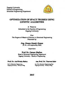
form subsequent generations. After several generations, convergence to an optimal solution is often accomplished. Determining the fitness of an individual is problem dependent and the fitness function usually incorporates a priori knowledge of the desired optimum. The basic genetic algorithm is improved by using problem specific knowledge in specifying the various operations required to direct the evolution. A discussion of the basic components will be given below in Section 2.2, followed by the incorporation of specific knowledge of first order saddle points in Chapter 3. Genetic algorithms have been applied to a very broad range of problems, in particular, problems associated with searching and optirnization. Increasing application complexity often requires larger and larger population sizes to sufficiently sample the search space and achieve a satisfactory solution. The terrninology associated with genetic algorithms is analogous t o that of biological systems. A generation is defined as one cycle of fitness evaluation, selection of parents, and reproduction. See Figure 2.1 for a flow chart of a genetic algorithrn, which will be described below. Individuals are usually represented by a single chromosome, given as a string of binary bits. Each bit represents a gene, and a given
expression of that gene (O or 1) is an allele. The bits of an individual encode the values for the variables of the problem, where the encoding scheme used is somewhat problem dependent and chosen by the irnplementor. The selection of parents generally involves a random choice among the most fit individuals of the population, in an attempt to propagate good traits through the
.-
Generate Initial Population Evaluate Fitness of Individuais I
/
Individual
Report Optimum Obtained
/
P Choose Two Parents
1
Perform Mutation
Enough
1
Choose individuais for next generation (incorporate previous best individual)
Evaiuate Fitness of Offspring
Figure 2.1: Flow chart for a Genetic Algorithm
population. The most fit individuals in the population tend to produce more offspring by being selected for reproduction many times. An individual's fitness value is determined by the evaluation of a problem dependent fitness function. The chromosome of an individual represents its genotype, while the fitness value represents its phenotype- Reproduction is perforrned by crossing over the chromosomes of the two
parents to form offspring, followed by occasionally mutating some of the bits (O
t, 1)
in the offspring. Reproduction accomplishes recombination of the genetic material, maintaining diversity in the population, thereby ensuring that the solution space is well sampled, and thus increasing the probability of obtaining an optimal sohtion. Finally, after reproduction has taken place, a sample of individuals must be chosen to form the population for the next generation. After several generations, those individuals in the population that are most fit will tend to dominate, and, provided the algorithm has been well designed, the average fitness of the population will increase. leading to convergence t o an optimal solution. The various operations in a genetic algorithm are discussed i n more detail in the following section.
2.2
Basic Principles
The operations in a genetic algorithm are dependent upon the probIem being solved, and many of the decisions are based on a combination of trial and error and previous experience. Some of the many ways to implement the various operators, and their advantages and disadvantages will be discussed. The detailed behaviour of
Figure 2.2: Example of forming a chromosome from encoded variables.
these operators, in turn, depend on several parameters, the values of which can lead to drastically different evolution. Hence, careful choices must be made. Previously
documented experiments can help in making these choices. Some of the parameters involved, along with some issues that may help in choosing values suited to a particular problem, are presented below.
2.2.1
Encoding
The chromosome string of an individual contains an encoding of that individual's solution to the given problem. The solution of most problems consists of a set of values defining the problem variables. The variables involved in optimizing a function f (z, y, z ) ?for example, are x, y, and z. The values of the problem variables are often
separately encoded as binary strings and concatenated to forrn the chromosome, as shown in Figure 2.2.
The encoding scheme, along with the fitness function, are
the two most important considerations for an efficient GA implementation. The encoding scheme is important when dealing with rea! life problems since a particular
Integer
Binary
Gray
Figure 2.3: Example of the Gray code characteristic that two successive values differ by one bit flip.
chromosome may represent an invalid solution. An effective genetic algorithm must take this into consideration in some way, whether it be within the encoding scheme or in the reproduction operators. A possible alternative to standard binary encoding is
Gray code. Gray code is similar to binary with the added feature that the Hamming distance. the number of bits that differ between the bit string representations of two adjacent numbers, is constant. In the case of Gray code, two successive integer values differ by only one bit flip, as shown in Figure 2.3. In most problems that require optimization' the variables involved are in real number space. Hence, the encoding scheme must also provide a way to store real number data in a binary string. The most common encoding scheme is interval (or range) encoding: where the domain and desired precision for the variables are specified initially, and the number of bits to be used for each variable is given by,
The scaled decimal equivalent (D) of each variable xi is given by,
where [ai, bi] is the domain of xi. The binary representation of this value is used as the encoded variable. The larger the number of bits used for each variable, t h e finer the resolution obtained for a given domain. An alternative to the interval encoding is multiplicative encoding where e a c h real nd truncated, where the accuracy i s detervalued variable is multiplied by 1 0 a c ~ ' a ca~ mined by the nurnber of accurate decimal places required in the solution. T h e binary representation of the resulting integer is used as the encoded variable. The encoded variables used throughout the evolution will normally be decoded (by reversing the encoding process) for fitness evaluation.
2.2.2
Initial Population
Generation of an initial population of individuals is often performed in a stochastic manner. However, for many applications, several infeasible individuals may result- It is generally better to generate a population using a prion' information of the optimum sought. For geometry optimization such as that being considered in this thesis, a pn'on'knowledge of a chemical reaction can lead to a reasonable guess a t the optimum. Thus, this initial guess provides a good starting point for the algorithm. One critical
factor is the number of individuals in the population, the population size, p, which can range from just a few individuals to several thousands. The population size is generally kept constant throughout the optimization. A rule of thumb for choosing p is 10 times the number of variables but no less than 100.
A population that
is too small will tend to give poor sampling and hence poor solutions, generally representing local rather than global optima. This concern is more detrimental for problems involving a large or convoluted search space, such as the optimization of proteins, which have complex structure and many conformations. However. there is usually a population size above which no improvement is seen, regardless of the number of generations completed. For the optimization of transition state structures. the initial geometry is usually relatively close to the optimum sought and hence the optimization is considered a local search. Wowever, given the accuracy that is required in the optimized geometry ( z 1 0 - ~ ) ,a sufficiently large population will still be required.
2.2.3
Fitness Function
The fitness function is the most fundamental component of a genetic algorithm. It is the sole mechanism for directing the evolution toward the desired objective. An individual's fitness value should represent how good of a solution t o the given problem it represents. The fitness function should take into consideration each variable to be optimized, and combine them in such a way to produce a suitable numerical fitness
value when applied to an individual. To ensure that the evolution is efficient, that is. the subsequent individuals are most likeiy to be biased toward better fitness values, the fitness function should contain few extrema, the ideal case being a monotonically increasing or decreasing function with a single maximum or minimum.
2.2.4
Selection
Selection is a means to favour the most fit individuals in the population in order to propagate good genes through the population. Some of the ways to select parents for reproduction are, roulette wheel selection, tournament selection, rank selection, sigma scaling, and Boltzmann selection. Although al1 methods use randomized processes, each has a n ordering scheme with which to bias the choice of the most fit individuals. Roulette wheel selection is equivalent to giving each individual a slice of a circle. with the size of the piece proportional to the individual's fitness. A point along the edge of the circle is randomly generated, and the individual whose slice of the circle contains this number is selected. Roulette wheel selection can cause problerns if one individual in the population is much more fit than al1 of the others. In this
case it can dominate the population resulting in premature convergence, that is, early convergence to a suboptimal solution. Tournament selection involves randomly choosing a number of individuals to take part in a tournament. The individual with the largest fitness in this tournament pool is selected for reproduction. A larger tournament size results in a higher selection
I I
Parent 1 :
O1 1 0 1 ~ 0 1 1 1 I
I
1
Parent 2 :
1 0 0 0 1:OlO I
Offspring 2 :
1 0 0 0 1 ~ 0 1 1 l
t
crosspoint
Figure 2.4: Application of the single-point crossover operator on 2, 8-bit individuals
pressure, which can be quantitatively viewed as the ratio of maximum to average
fitness values of the current tournament. Selection pressure can also be increased by using a probabilistic tournament selection. In this case, the best fit individual in a tournament is selected with a user defined probability. A larger probability results in
a higher selection pressure, a probability of 0.5 represents no selection pressure. Too high of a selection pressure leads to fast convergence to solutions that are suboptimai. while too low of a selection pressure leads to long execution times for convergence.
2.2.5
Crossover
Crossover is used as a means to generate better individuals than those that were present in the population previously. Two individuals are chosen as parents, their bit strings are aligned, and a crossover point is chosen randomly (see Figure 2.4). The strings are then crossed by exchanging the bits to the right of the crossover point, forming two new individuals. The crossover just described is called single-point crossover. Multi-point crossover can also be used, and is irnplemented in a simiIar
Offspring 1 :
Mutating Bits
Offspring 2 :
-
Figure 2.5: Application of the mutation operator on offspring produced by crossover
way. swapping portions between crossover points. Crossover is performed based on a user defined probability, p,, which is usually set between 0.60 and 1.0. Hence,
some parents pass on their genetic information directly to their offspring, without modification by crossover.
2.2.6
Mutation
Mutation is used t o maintain diversity in the population. Although it does not necessarily generate better individuals, mutation prevents stagnation in a population of like individuals, which otherwise may not evolve to an optimum. The genes chosen for mutation have their state reversed by changing 0's to l's, and 1's to 07s,as required (see Figure 2.5). Mutation is performed with a user defined probability, p,, usually set very low (0.001
-
which is
0.01) to prevent a large disruption of the genes in the
population. A mutation probability of 0.5 results in the generation of offspring in a rnanner akin to a random walk. The issue to be addressed when choosing a mutation rate is to strike a balance between destroying good genes and using mutation as a
beneficial search operator. Too high of a mutation rate results in a n undirected search, while too low of a mutation rate can lead to premature convergence or stagnation. Gray code can sometimes help moderate mutation effects in this respect, since one bit flip changes the number by the smalest integer amount, regardless of which bit is flipped. In c o n t r a t , flipping a more significant bit in standard binary results in a big change in the variable value.
2.2.7
l
Incorporating Offspring
After reproduction is complete, X offspring and p
-X
parents must be chosen to
become the population for the next generation. Since sorne of the offspring may be less fit than the parents, most implementations choose a combination of offspring and parents for the next generation. To bias the evolution toward the desired optimum, the most fit of the two groups can be chosen, until the required number of individuals is reached. Hence, the most fit of the offspring replace the l e s t fit of the parents.
It is normal for the single best individual from the previous generation t o be copied back into the population for the next generation. This practice is known as elztism. 'An example of the effect of flipping a single bit in standard b i n a q versus gray encoding is shown. where the value 1.54 is encoded by multiplying by 10% The original binuy strings as well as the result of Aipping a single bit are shown. Encoding Binary Gray
Bit String
Mutated
Decoded Value
10011010 11010110
00011010 01010110
0.26 0.86
Note the much larger ciifference that results fiom flipping the most significant bit of the binary encoded variable compared to the Gray encoded variable.
Met hods for incorporating offspring can becorne rather sophisticated and Vary widely.
2.2.8
Convergence
For the purposes of optimization, genetic algorithms are usually terminated when the solution has converged. Convergence can be determined in several ways. One common method is to terminate evolution when the quality of the solutions have not improved for a number of generations. Yet another, is to terminate when a given individual, with a high fitness value, has occurred a number of times. In general. evolution can also be terminated after a user defined number of generations has evolved. As the algorithm converges, the average fitness, and the fitness of the best individual increases, wit h the average approaching the highes t fitness value as the optimum is reached. It is likely that some problem specific variable couId be used to determine convergence.
2.3
Why Genetic Algorithms Work
When considering the question of why GA'S work one must not forget that genetic algorithms were modelled after natural biological processes, which have proved their efficiency as demonstrated by
Our
own human evolution.
Following the development of practical application details, the theoretical foundations for why genetic algorithms are able to mimic nature should be addressed. The basis for a formal rneans to do this was provided by John Holland [22], who introduced
the schema theorem. A schemata is defined as a bit pattern that is represented as a binary string of O's, 1's' and r's, where a + is a "don't care" symbol, and can thus represent a O or a 1. A given chromosome contains many schema. For example, the chromosome 1101 contains the schema I l
* *, 1 * 01, etc.
Two properties of schema
are: The order of a schemata, which is the number of static bits, or the number of non-* bits. The defining length of a schemata is the distance between the furthest static bits. For each generation, individuals are considered for reproduction, with higher fit individuals more likely to pass on their traits to the next generation. Since selection is based on fitness, and one assumes that higher fitness values are a direct result of good schema, the representation of good schema in the population should increase exponentially in successive generations. These are the ideas of Holland's schema theorem. As an implication of this theorem, if one considers the number of schema compared to the number of individuals, the ratio is very large. According t o Holland. the number of schema processed for each generation is oc
p 3 , where
p is the population
size. In addition to Holland's scherna theorem, a well-known approach by Goldberg
[23], called the Building Block Hypothesis, also attempts to explain why GA'S work. Goldberg defines the term building block as a "highly fit schemata of low defining length and low order." The idea behind the building block hypothesis is that, in a
GA, convergence to the optimum occurs because of the placement of building blocks.
This hypothesis leads to encoding criteria for efficient performance of a genetic algorithm. These criteria include pIacing related genes close together in the chromosome. and having little interaction between the genes. If both criteria are satisfied the effectiveness of the GA is determined by the schema theorem. However, these criteria are d f i c u l t to satisfy. In the majority of cases there is some interaction between genes. that is, the amount that a given gene contributes to the fitness value depends on the value of its interacting gene(s). Satisfaction of both criteria is a1so snagged by lack of a priori knowledge of interaction between genes, and, in order to fil1 the first criterion, the second must be met. The best resort is to corne as close as possible to satisfying Goldberg's encoding criteria. As part of this thesis, an impiementation of genetic algorithms for optimization
of chemical structures was written in C, interfacing with Fortran 90 in the Mungauss package. Details of this implementation can be found in Appendix A. Chapter 3 presents results and a discussion on parameter selection.
Chapter 3
Results From Mat hematical Funct ions "In theory, there as no diflerence between theory and practice. In practice there is." -UnLnown
In this chapter a discussion of the resuIts obtained from the optimization of mathematical functions using genetic algorithms is given. The purpose of these results is to demonstrate the effectiveness of the algorithm as well as to analyze its behaviour.
3.1
The Sample Problem
Two-dimensional mathematical functions provide a good testing medium since their surfaces are easily constructed and their stationary points can be visualized. This is unlike chernical reactions, where the surface is not known, and in most cases neither are the stationary points. As a means of testing the genetic algorithm code implemented, the following mathematical function given by Chong and Zak [24] was
1
Y
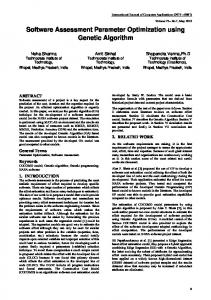
Figure 3.1: Surface of the Chong-Zak function given in Equation 3.1.
used,
whose surface is shown in Figure 3.1'.
This function contains two minima, three
maxima, and three saddle points, as can be seen in Figure 3.2. The coordinate values and characteristics of these stationary points are listed in Table 3.1 For the given objective function two fitness functions were constructed appropriately to seek out both minima and first order saddle points respectively. Note that lThis surface l o o k slightly different from the one mistakenly shown in [24]. Despite this fact, the function used here is identical to the one stated in the reference. Furthermore, the authors of [24] identify the stationary points of their imaged function, not of the function given in the text. However, the correct stationary points for Equation 3.1 are given in this text in Table 3.1.
Location of Stationary Points 2 minima. 3 maxima 3 F i t order saddle points
Figure 3.2: Contour plot of Equation 3.1 showing minima (m), maxima (M), and saddle points (x) (see Table 3.1). The stationary points are labelled for future reference.
Table 3.1: Location and characteristics of the stationary points for the Chong-Zak function. (x, y) is the coordinate location, f (x,y) is the function value, 11911 is the gradient length, Al and X2 are the eigenvalues of the Hessian matrix. Note that llfll would be exactly O a t the stationary points if calculated analytically. x Y f (x,Y) 11d1 AI A2 label ml -1.431359 0.206945 -2.467838 3-246533 x 1W6 7.4497 14,3481
no higher order saddle points exist for the current function since f : IF?
3.2
*R
Fitness Evaluation
Since the ultimate goal is to optimize first order saddle points on a potential energy surface, a fitness function was designed to isolate the desired features of such stationary points. As noted previously, first order saddle points can be characterized by a zero gradient and one negative eigenvalue in the Hessian matrix. With this in
mind, the following fitness funct ion was developed,
where I is a vector of the problem variables, divided by
fi where
llijll is the 12-norm of the gradient vector
k is the number of problem variables (or gradient length), n
is the number of negative eigenvalues in the Hessian matrix, and
E
is a parameter
chosen smal12 and used to prevent division by zero as the algorithm converges. Note that individuals that are close to a first order saddle point (11911 h: O, n = 1) will have higher fitness values than those further away since their gradient norm and number of negative eigenvalues will result in small denominators in the fitness function. Hence, the genetic algorithm should be constructed to positively bias those individuaIs wit h 'The parameter E is chosen to be on the order of the desired accuracy in the gradient length of the converged solution. A value of L x 10-6 is used since this is somewhat of a standard for convergence in chemicai structure optimization.
the highest fitness values. Wit h this fitness function, a n "optimum1 solution corresponds t o a first order saddle point- Note that this fitness function does not bias one saddle point over another, therefore the algorithm could theoretically find al1 or any of the first order saddle points on the surface. For the optimization of minima the (n- 1) term in Equation 3.2 was changed to n such that individuals with al1 positive
eigenvalues would be favoured. Various runs of the genetic algorit hm, performed with different parameter values, are discussed in the remainder of this chapter to illustrate the behaviour of the method, and its dependence on these parameters.
3.3
The Defining Parameters
Several parameters characterize and control the operations of the genetic algorithm and affect the behaviour of the evolution towards an optimum. These parameters are listed in Table 3.2 below. Although many of these parameters were discussed briefly in Chapter 2, a few require further explanation.
An initial population of
individuals is generated by taking small random perturbations about an initial guess at the optimum. These perturbations are restricted by the value of Minit since it
is assumed that the initial guess is a good one. Furthermore, since the problem to be solved typically involves data for a physical system, the individuals created throughout the evolution are restricted to within Msub of the initial guess to avoid infeasible values.
Any individuals that fa11 out of this region are forced back by
changing the invalid variable values to small random perturbations from the initial
Table 3 -2: Parameters in the current genetic algorithm implementation. Notation Description Initial guess a t the optimum. Population size. Maximum number of generations. Probability of crossover. Probability of mutation. Number of bits per variable. Maximum amount t o perturb the initi.al guess tlO form the initial population. Maximum amount any subsequent individuals can deviate from the initial guess. Method used for selecting parents. Possible values are 't' for tournament selection and 'r' for roulette-wheel selection. For tournament selection, parameters include the size of the tournament, tSize,and the probability of selecting the most fit individual, troa. Type of encoding scheme used. Possible values are 'm. for multiplicative and 'i' for interval (or range). Binary representation used. Possible values are 'g7 for Gray and 'b' for standard binary. Type of replacement strategy used to form the population for the next generation. Possible values are 'a' for aboveaverage and '0' for all-offspring. The value beiow which negative eigenvalues must lie to be counted as negative.
guess, as before. Following the completion of each generation, forming the surviving population for the next generation can be done in two ways. First, the population can be formed from only the offspring created in the current generation. Second. the population can consist of random selections from among the parents and offspring that have above average fitness values. In the latter case, the best individual from the previous generation is always copied back into the new population. The parameter
R specifies which of these methods to use. Finally, .Ator is a tolerance that is placed
on the value of the negative eigenvalues, below which they must lie to be counted as negative. This parameter is required because of finite machine precision which can cause values that are essentially zero to be very small, and maybe negative. Points with such negative eigenvalues are of no interest, but nevertheless would be considered favourable by the fitness fuaction. For the Chong-Zak objective function this can cause problems a t points in the flat region of the surface (outside the interesting regime) where the gradients are srnall and one of the eigenvalues is small and negative.
In this case XtOl = -5.0 has proved to be adequate to concentrate the search in the interesting region of the surface.
3.4
Results for First Order Saddle Points
The following subsections investigate the effect of each of the parameters in the algorithm. Since genetic algorithms are stochastic in nature, each run represents only one sample out of the total ensemble. Thus, to obtain statistically significant results data was taken over 25 runs for each parameter set and averaged. For each of these runs a different random seed was used and recorded. Subsequent data sets were generated using these same 25 seeds for consistency. For the current analysis the default parameter values are as follows: xo = y0 = 0.0, ,u = 100, Gm,, = 200. pc = 0.75, Pm = 0.03,
nb
= 24, Minit = MSub= 2-07 S = 't,' tSize = 6, tprd = 0-75.
E = ' m l 1B = 'g,' R = 'a,' the respective figures.
= -5.0, with any differences noted in the captions of
3.4.1
Location of the Initial Guess
Since the initial population of individuals is created by perturbing an initial guess a t the optimal variabIe values, the exact location of this initial guess can have a profound effect on the behaviour of the algorithm. Figure 3.3 shows the effect on the average and best fitness values resulting from changing the initial guess from (O. 0) to (-1, -1), with Min,, = Msub = 3.0 such that both cases encompass al1 of the interesting region of the surface. There is little difference in the overall behaviour
Average and Best Fitness Values Effect of Changing the Initial Guess
b
average (xo=yo=O) best (xo=yo=û)
best (xo=yo=- 1 )
1
I
50
1
I
100
1
I
150
I
2
generation
Figure 3.3: Plot of average and best fitness values for different initial guesses. The case with (xo,go) = (0,O)results in slightly better fitness values.
of the algorithm due to changing the initial guess, since the average and best fitness
Table 3.3: Results obtained by varyïng the initial guess, where Ga, is the average nurnber of generatioos required t o find the best individual found in the evolution. Initial Guess Region (a;, Y) Ikdl n Gau, ( O l 0) 372 (1.148302,0.868567) 3.462192 x 10A6 1 84
values follow similar trends. However, the case with initial guess (-1, -1) gave higher fitness values slightly earlier. Furthermore, the two cases report optima in different regions of the surface as shown in the results in Table 3.3. Initial guess (O, O) resulted in a nearly equal number of optima cear
x2
and
x3
(see Figure 3.2). In addition, one
of the runs for (xo,yo) = (O7O) resulted in premature convergence to a suboptimal solution. Initial guess (-1, -1) resulted in the majority of optima near x3, with a significant number of optima also found near
x3, in
an average generation of 6 3 . In
addition to the difference in time required to cluster around a point, the initial guess can have a direct influence on the location of the optimum found, as is to be expected.
3-4.2
Effect of Perturbation and Validation Parameters
For the current genetic algorithm design, the parameters Mi,it and Msubdirectly affect the behaviour of the algorithm and are closely linked with the location of the initial guess. A plot of the best fitness value each generation for initial guess (-1, -1) and different Minit and Msub values is shown in Figure 3.4. Again, the overall behaviour is similar, but with Minit = Msub = 3.0 resulting in a slightly
Best Fitness Values
Cornparison of Different Minitand MSu,Vdues
generation
Figure 3.4: Plot of best fitness values for different values of Minit and Msub. The case with Minit = Msub= 3.0 gives slightly better fitness values.
better fitness value. However, the three sets of runs again result in different optima. Parameter values Minit = MSub= 2.0 resulted in the majority
O&
optima near xl in
an average generation of 63 but with 4 runs converging prematur-ely. The set of runs with Minit = 2.0, Msvb = 3.0 resulted in the rnajority of optima n e a r
XI
as well, but
in an average generation of 55 and no runs converging prematurely. The set of runs with Minit = Msub = 3-0 resulted in the majority of optima near generation of 60, but did not report any optima near
xl.
x2
in an average
It is important to note
that with (xo,yo) = (-1, -1) and Minit = MSub= 2.0, the only s a d d l e point within
the region defined by the M,it
and Msub constraints is zl. Clearly, the optimum
obtained is highly dependent on the value of Mhit and MSubsince srnaller values of these parameters result in a more local search.
3.4.3
Effect of Population Size
To demonstrate the effect of population size on the outcome of a genetic algorithm, two cases with p = 100 and p = 200 are displayed in Figure 3.5. Results obtained
Average and Best Fitness Values Cornparison of PopuIation Size
.--*..-average (p=200)
bes t (p=200)
Figure 3.5: The effect of population size on the behaviour of the genetic algorithm. Doubling the population size has little effect, but does result in slightly earlier convergence.
for these sets of runs are shown in Table 3.4, where the percentage of runs resulting
Table 3.4: Results obtained for different population sizes, where p = 200 found an optimum slightly earlier on average than p = 100. Region % of runs Ga,, 100 200 100 200 Xl 22
X3
8
4
28 64
56 40
49 57 57
33
46 49
in optima near each saddle point is shown. Note that both sets of runs resulted in optima near al1 three saddle points. Doubling the population size makes very little difference, with the exception that the Iarger population gives earlier convergence on average. This is likely because the sampling of the surface is more thorough with the larger population, and it is therefore more likely to have individuals with high fitness values early in the evolution. One very important factor in considering the usefulness of doubling the population size is the increase in computational overhead associated with more individuals. It would seem reasonable to assume that the improvement in behaviour with the doubled population would not be worth the expense unless the optimum was found in half the number of generations. For the current example this is not the case so doubling the population size is not likely to be worthwhile.
3.4.4
Effect of Crossover Rate
The effect of changing the crossover rate is shown in Figure 3.6 where the average and best fitness values are displayed for p, = 0.60, 0.75, and 0.90. Results obtained
Effect of Crossover Probability pc=û.60,0.75,0.90
----
average (pc=0.60)
- best (pc=0.60) -...... average (pc=0.75) .-.- best (pc=0.75) .-..- average (pc=0.90) -.-- best (pc=0.90)
Figure 3.6: The effect of changing the crossover probability p, with standard binary encoding. A crossover probability of 0.60 results in higher fitness values but gives slower convergence.
for these sets of runs are shown in Table 3.5. Note that al1 three values of p, resulted in optima near al1 three saddle points, but somewhat faster convergence is achieved with pc = 0.75. In addition to the runs performed above one sample run of the algorithm with p, = 0.60 resulted in premature convergence. A scatter plot of the individuals present
every 40 generations during this run is shown in Figure 3.7 where the algorithm forms two clusters near Ms , ultimately favouring individuals in the cluster near x3,yet never act ually reaching the optimum.
Table 3 -5: Results obtained for different crossover probabilities, showing p, = 0 -75 reporting an optimum slightly earlier% of runs Gaug Region
x3
For the Chong-Zak function we conclude that p, = 0.75 appears to be the best crossover probability due to faster convergence on average.
3.4.5
Effect of Mutation Rate
Thus far, most runs of the genetic algorithm reported a majority of optima in the region of the surface near saddle points
x2
and
23,
however there are three saddle
points present. Once a good individual is found, al1 subsequent individuals seem to move in that direction and cluster within small regions3. In cases where the initial guess is a good one this is a desirable behaviour, since the clustering will most likely occur around the optimum sought. This effect can be seen in Figure 3.8 in which the individuals are displayed every four generations for the first twenty generations of a sample run. To prevent this rapid clustering, in the hope of finding the other saddle point, the mutation rate can be increased to ensure more thorough sampling of the surface, Figure 3.9 is a scatter plot generated by increasing the mutation rate --
-
3There is a possibility that such clustering can actuaiiy Iead to problems due to premature convergence. Later work by the author addressed this concern, and a discussion can be found in Section 4.4.
Scatter Plot of Individuds Demonsuation of Premature Convergence 0-3
1
I
1
I
1
I
I
I
x parameter
Figure 3.7: Scatter plot of individuals every 40 generations for p, = 0.60, where each point represents a single individual in the population. This r u n demonstrates premature convergence. The location of the two clusters relative to the stationary points on the surface is sho- on the super-imposed contour plot.
from 0.03 t o 0.08. Note that there is distinct clustering around both saddle points x2 and x3 (regions A and B of Figure 3.9 respectively), but with much more dispersion than with p , = 0.03. However, the best individual was still found near
(x, y) = (1.148302,0.868567), llijll = 3.462192 x 10⁻⁶ and n = 1.
X Q , with
x parameter
Figure 3.8: Scatter plot of individuals every 4 generations for the first 20 generations, with p, = 0.03. The population quickly clusters around saddle point x3 in region B. The optimum reported was x = 1.154115,y = -0.890394, where IlG[l = 1.581266 x 10⁻⁶ and n = 1. Enlarged views of areas A and B are shown in the graphs on the right .
3.4.6
Effect of the Selection Method
To compare the various available strategies for choosing parents for reproduction, the two implemented methods are compared in Figure 3.10. Two cases using tournament selection are shown with different selection pressures4 imposed by changing the number of individuals taking part in each tournament. Although there is little differ4see Section 2.2.4
Scatter Plot of Individuds mutation probability=0.08
x parameter
Figure 3.9: Scatter plot of individuals every 4 generations for the first 20 generations with p, = 0.08. Although the optimum reported was in the region of x3 (B), the sampling continues to cluster around x2 (A) as well. Enlarged views of regions A and B are shown in the graphs on the right.
ence between the three plots, roulette-wheel and tournament selection with tsi,, = 6 behave very similarly, while tournament selection with tsiz, = 2 does not perform as well. Examination of the optima obtained reveals the same conclusion, as shown in Table 3.6. Note that neither S = Y ' , tsize= 2 nor S = 'r' found
X I , and
that S = ' t ' ,
tsi,, = 6 gave results earlier than either of the other two methods. Hence, S = 't', t,,, = 6 appears to be the best selection method of the three tested. However, one must also consider the slight increase in overhead associated with
Cornparison of Parent Selection Methods Roulette-wheet and Tournament
100
generation
Figure 3.10: A comparison of roulette-wheel and tournament selection. Two runs of tournament selection are shown with different selection pressure, changed by using 2 individuals in each tournament instead of 6.
increasing tSize from 2 to 6 since there are 3 times more cails to choose random individuals from the population, as well as 3 times more comparisons of fitness values to determine the most fit individua15. Regardless, it is thought that the improvement in evolution speed is worth the small expense. 'sec Section A.3.1
Table 3.6: Resdts obtained for different parent selection methods. Note that S = 't' with tsize= 6 gave earlier results and is the only method that finds saddle point XI.
3.4.7
Effect of the Encoding Method
The effect of changing the encoding method from multiplicative encoding to interval (or range) encoding is shown in Figure 3.11 which plots the average and best fitness values for both types of encoding. Interval encoding was used with nb = 22 for the intervals x, y E [-2,2] since a precision of 0.000001 is desired (see Equation 2.1). Therefore, to ensure a fair comparison, multiplicative encoding was used with nb = 2 1 since the largest number to be encoded is 2.0, requiring a representation of at most 2 x 10% For multiplicative encoding only x2 was found, with gradient lengths on the
order of
in a n average generation of 50.1. Whereas for interval encoding a11 three
saddle points were found with gradient lengths on the order of
but slightly less
than multiplicative, in an average of r=: 55 generations. As a result, interval encoding is considered superior to multiplicative encoding since a slightly more accurate result was found with minimal increase in the number of generations and the problem space
was better sampled, since al1 three saddle points were found.
Cornparison of Encoding Schemes Multipiicative and Interval (or Range)
generation
Figure 3.11: A comparison of multiplicative and interval encoding. The interval encoding method outperforrns the multiplicative method since a slightly higher fitness value is attained, and al1 three saddle points are found as opposed to just x2 for multiplicative encoding.
3.4.8
Gray versus binary
The encoding scheme is also defined by a choice between standard binary or Gray
encoding. A comparison of the use of Gray encoding versus standard binary encoding is shown in Figure 3.12. Note that both sets of data follow the expected trend of the average fitness approaching the best fitness as the algorithm evolves. The Gray encoding performs much better, reaching an optimum after an average of
= 54
generations. The standard binary encoding however, levels off at a much lower fitness
Cornparison of Gray and Standard Binary Average and Best Fitness Values 1
m
I
I
I
I
1
d
average (B=g) best (B=g)
1
r
----.-*
average (B=b) best (B=b)
-
-
generation
Figure 3.12: Plots of average and best fitness values for Gray and standard binary encoding. Gray encoding far outperforrns standard binary encoding.
value. In addition, while t h e optima found in both cases contained one negative eigenvalue in the Hessian, t h e Gray encoded algorithm resulted in optima al1 with gradient lengths on the o r d e r of
Whereas, the standard binary encoding only
resulted in one run (out of 2 3 ) with an optimum with such accuracy. Clearly, Gray encoding proved to be the b e s t encoding scheme for this example. This result was somewhat expected since G r a q encoding is less sensitive to mutation effects, resulting in a more gradual, and s m o o t h evolution6. %ee Section 2.2.6
3.4.9
Replacement Strategies
The final parameter t o be investigated is the method used to replace the individuals in the population from one generation to the next. Using only the offspring to form the population for the next generation can sometimes cause problems if many of the offspring are Iess fit than the parents. A plot of the average and best fitness vaIues resulting from using the all-offspring replacement and the above-average replacement is shown in Figure 3.13. Note that for R = 'O' the average fitness values remain noisy
Effect of Replacement Strategy Cornparison of above-average and ail-offspnng 1
I
I
.
L
I
I
.
*
.
.
I
--
I
.:-.
- - = -- ...=.. .. . "- - -
. ---' - --..- .....=t... -i
average (R=a) best (R=a) .- ..... average (R=o) best @=O)
: -
generation
Figure 3.13: Plots of average and best fitness values for above-average(R = ' a ' ) and all-oflspring (R = '0')replacement strategies. The all-offspring strategy results in the average fitness values never approaching the best fitness values.
throughout the evofution, never approaching the best fitness as is expected. This is due to the stochastic nature of the offspring creation and the resulting lack of bias when using them as the new population. Examination of the individuak present in the population show that many individuals far removed frorn any first order saddle point remain in the population throughout the evolution, weighing down the average. This can be seen in Figure 3.14 where the contours of the function are superimposed
Scatter Plot of Individuals
x parameter
Figure 3.14: Scatter plot of individuals for all-o#spring (R = ' O , ) , displaying clustering around saddle point xs.
on the graph. An interesting feature to note is that many of the individuals have the same
x value, and many have the same y value. This phenomenon is due to single-point crossover, since this f o m of crossover changes only the variable in which the crossover point occurs, leaving al1 others the same. Hence, as the algorithm evolves and favours a given stationary point, most of the offspring formed will contain changes in only one of the problem variables, hence creating vertical and horizontal lines on a scatter plot (as seen in Figure 3.17) intersecting near the optimum. This effect would be diminished by increasing the mutation rate, causing many, or all of the variables to be modified in many of the offspring produced.
3.5
Objective Function Geometry Considerations
To explore how each of the runs for a particular set of parameter values contribute to the overall average obtained, a plot of the average fitness value of each generation for each run was plotted along with the overall average. This plot is shown in Figure 3.15 where the dots are the average fitness values for different runs and the solid line is the overall average of these average fitness values. Note that three distinct bands of points occur. Each of these bands corresponds to populations sampling the areas around different saddle points on the surface. In other words, sampling the region surrounding different saddle points can result in a different average fitness value for that sample. This phenomenon is a consequence of the encoding scheme used and the local geometry of the surface around the stationary points. The use of a particular encoding scheme is equivalent to defining a grid of discrete values on
Contributions to the Overall Average Overall Average and Average Fitness Values for 25 runs
generation
Figure 3.15: Plot of average fitness values each generation for each of 25 runs with the overall average of these runs. Three bands of points correspond to the three saddle points on t h e surface.
the surface of the objective function from which the variable values can be chosen to form individuals. To illustrate, consider a surface whose contours are shown in Figure 3.16. This surface displays two maxima of the same height , with maximum A laying atop a gently sloping hi11 and maximum B laying atop a steep slope. The same grid size, representing possible discrete values of a sample, is superimposed on both of these stationary points. Note that the objective function values under the grid a t
A do not change nearly as much as the objective function values under the grid a t
B. The fitness values will follow this sarne trend. Thus, a point on the grid a given
Figure 3.16: Contours of a sample surface to demonstrate the effect of the local geometric features of the objective function. The surface around maximum A h a a more gentle slope than the surface around B which is a steep maximum.
srnall distance from the maximum a t A will have a lower gradient than a point the same distance from the maximum a t B. For the fitness function used, this will result in samples taken near A having a higher fitness value on average than sarnples taken
near B, provided each has the same number of negative eigenvalues. This is reflected in Figure 3.15. However, taking the log of the fitness values (as was done throughout this chapter) results in the three bands of points collapsing together around the overall average line. Consequently, any difference in fitness values seen on a log plot are significânt, and not due t o landing on different stationary points.
3.6
Results for Minima
To illustrate the robustness of genetic algorit hms for optimization problems, the fitness function was modified, whiie maintaining the same basic structure, to seek the minima of the Chong-Zak function. The behaviour exhibited was similar to that seen for saddle points.' A scatter plot of individuals for a given run is shown in Figure 3.17, where the first minimum, mi is found a t (x,y) = (-1.431359,O-206945),
Ildl
=
3.246533 x IO-^, n = O in generation 99. The all-offspring replacement method was used here since it allows one to easily observe the convergence.
Scatter Plot of Individuals
x parameter
Figure 3.17: Scatter plot of individuals for /I = 200, B = 'b,' with the fitness function chosen to seek a minimum.
R = 'O,' and AM
= 0.0,
In another plot where the population size was decreased to 100, with B = '9' and R = 'a' ma happened to be obtained.
The optimum found was a t ( x , y ) =
(0.404936,0.166523), with f (x,y) = -0.930778, [lijll = 1.703883 x 1 0 - ~ in generation
59.
3.7
Conclusions and Recornrnendations
As a result of the above testing performed on the Chong-Zak function, the recommended parameter values for efficient use of this implementation of a genetic algorithm are: p = 100, G,,
= 200, p, = 0.75, p,
= 0.03, nb = 24, S = 't,' tsiie = 6 ,
tPob = 0.75, E = 'i,' B = 'g,' R = La.1It is concluded that these values gave the best results in general and provide a good starting point for the optimization of transition state structures'. However, given the large increase in computational complexity in moving from 2D mathematical functions to chemical structures, it is likely that G,,
= 200 will result in long wait times. T h i s is not likely to cause problems since
most runs of the algorithm with B = 'g' showed little improvement after G,,,
= 100,
hence 100 generations will be used as the s t a h n g point. Also, Minit, Adsub,and At,[ are problem dependent and would therefore b e very different for chemical structures. Note that a convergence criteria should be introduced since the possibility of obtaining a more accurate solution in subsequent generations should be balanced with the -
-
-
'Note that these parameters are not completely indeyendent, and some coupling exist between many or all of the parameters. Hence, a more thorou& investigation of the effect of the parameter values on the behaviour of the algorithm would include many more combinations of possible values.
expense of continuing the computation. Thus, for chernical structures the convergence criteria,
11ijIJ< b is introduced, where b is user
as the default value.
defined. We will choose 6 = 5 x 10⁻⁵
Chapter 4
Results From Chernical Structures "No arnount of experimentation can ever proue me right; a single experiment can proue me wrong." -Albert Einstein
The transition from the optimization of mathematical functions to the optimization of chernical structures requires the consideration of several additional concepts. One consideration is the choice of coordinate system to use. Interna1 coordinates in the form of a Z-matrix was used as it provides the most intuitive structure description.
In 2-matrix coordinat es, one represents the molecule by the bond lengths between adjacent atoms, and the angles between adjacent bonds. Other common coordinate systems include Cartesian where each atom is simply assigned its position in xyzspace, and natural interna1 coordinates which represents a structure as combinations of bond lengths, bond angles, and torsions. In GA'S, reducing the coupling between variables is preferred since this allows them to evolve independently and leads to a more efficient algorithm. Based on the amount of coupling between variables, Z-
matrix coordinates are a good choice. In comparison to Cartesian coordinates and natural internal coordinates, 2-matrix coordinates have less coupling than Cartesian coordinates, but natural internal coordinates provide nearly completely decoupled variables. Thus, future work on this project could possibly benefit from the use of natural internal coordinates. Second, one must decide on the method of energy calculation used. The energies, first derivatives, and numerical second derivatives were calculated using a n ab initio approach a t the Hartree-Fock level, with the 3-21G basis set. To demonstrate the viability of the genetic algorithm code, various transition state structures were selected for optimization. These choices were taken from a range of chemical reactions so as to sample some of the different chemical characteristics that can arise. The test cases shown in Table 4.1 were taken from the list provided by Baker and Chan [25] where a large variety of chemical reactions used in recent literature for test ing transition state structure optimization met hods are presented.
4.1
Physical Aspects of Transition State Structures
Recall t hat the defining characteristics of transition state structures, and t hus the features that should be isolated in a genetic algorithm are; transition state structures are first order saddle points on a potential energy surface whose second derivative matrix has one and only one negative eigenvalue, the gradient vector at these points has a norm of zero. Additionally, the eigenvector corresponding to the negative
Table 4.1: Test cases used for transition state structure optimization (Bond lengths a v e n in angstroms and bond angles in degrees). The starting geometries used for the current optimization are as shown in the form of a Z-matrix, and are the same as those given in [25]. 1. HCN tt HNC
2. HCCH
t,
CCH2 u
4. HNC
+ H2
H2CNH
t)
eigenvalue must be such that the deformation of the molecular structure in that direction along the surface connects the transition state structure to reactants and products.
4.2
Unique Features of the Genetic Algorithm
Unlike other transition state optimization techniques, the genetic algorithm approach is not sensitive to the structure of the initial Hessian. The algorithm promotes the production of individuals with one negative eigenvalue, favouring the correct Hessian eigenvalue structure. Furthermore, genetic algorithms are known for their ability to efficiently sample
a search space to locate a global optimum. Although this is not the intention in the current implementation it is worth noting that transition state structure optimization is less of a local search than the optimization of minima; for transition states. it is
very unlikely that an initial guess can be made as close to the desired optima as is possible for minima.
4.3
Results
For the optimization of chemical structures, the following parameter values were used: p = 100, G,
= 100, p, = 0.75, p,
= 0.05,
nb
= 31, S = Y', E =
'2'.
B = ' g ' , R = 'a', AtOl = 0.0. Some of these values differ from the starting values proposed in Chapter 3, which reflects the problem dependency of genetic algorit hms.
The mutation probability was increased from 0.03 to 0.05 since the former did not sufficiently sample the search space. The number of bits used for each variable, nb was increased to 31' since, for interval encoding, the accuracy increases with more bits. Since the negative eigenvalues for chernical structures are usually very small compared to those for mathematical functions, XtOl was changed to 0.0. Thus any negative eigenvalues, regardless of the size, are counted as negative. Furthermore, the generation of the initial population was modified for interval encoding. Individuals are generated randomly within the intervals specified for the variables, with the initial guess added to the population without modification. This eliminates the need for the Minit and Msub variables since al1 nb-bit integers can be mapped into t heir corresponding intervals, and t hus any subsequent individuals are guaranteed to be within the respective intervals. The structures given in Table 4.1 were optimized with the VA method discussed in Chapter 1, and the results are compared to those obtained from optimizing with
the genetic algorithm. Reaction 1 (see Table 4.1) is an HCN
tt
HNC rearrangement
and the results obtained are shown in Table 4.2. The bond lengths are reported in angstroms and the bond angles in degrees. The optimized structures obtained from both methods are very similar and both have a Hessian matrix with one negative The total energy, Et is reported eigenvalue and a gradient length on the order of 10-~. l This is the maximum number of bits that can be used for each variable since a single unsigned integer is used, corresponding to 32 bits, and a single bit is reserved for the sign bit, as in multiplicative encoding, despite the fact that it is not used in interval encoding.
Table 4.2: Results obtained for the HCN tt HNC rearrangement showing the initial geometry and the optimized geometries fiom the GA and VA methods. The Hessian has one negative eigenvalue (n) for al1 three structures, but the genetic algorithm structure has a slightly lower gradient length ([16[1) Variable Initial GA VA
Table 4.3: Results obtained for the HCCH t,CC& rearrangement showing the initial geometry and the optimized geometries from the GA and VA methods. The Hessian has one negative eigenvalue (n) for al1 three structures, but the genetic algorithm structure has a slightly lower gradient length (11ij11). Variable Initial L1 1.24054 1.65694 1.06318 60.3568 60.3568 -76.265417 2.68 x 10⁻¹ 1
in Hartrees and the initial and final values match those reported in [25]. Th-1s rea provides a good visual example since it only has three variables so a cluster plot can therefore be produced. An example of such a chster plot of individuals every 40 generations is shown in Figure 4.1. Note that the individuals cluster in a smaller and smaller region as the population evolves to the optimum. Results for Reaction 2 are shown in Table 4.3. The two optimized geometries are
Figure 4.1: Cluster plot of individuals every 40 generations for the HCN t, HNC reaction. The clustering of individuals gets tighter as the population evolves.
Table 4.4: Results obtained for the HOCI tt HC1 + CO reaction showing the initial geometry and the optimized geometries from GA and VA. The two optimized geometries are similar with comparable gradient lengths, with the VA gradient length slightly lower. Vari able Initial GA VA 1.11608 1.11607 L1 1.17 L2 2.335 2.55176 2.55180 1.10407 1.10418 L3 1.127 Al 90.0 126.6372 126.6381 A2 90.0 47.6255 47.5872 Et -569.57865 -569.89752 -569.89752 11911 4.58 x IO-' 4.73 x IO-^ 6.67 x 1od5 1 1 72 1
again very similar, both having gradient lengths on the order of IO-*. Again' the energies match those reported by Baker and Chan. Results obtained for Reaction 3 are shown in Table 4.4. There are only slight differences between the two optimized geometries and both converged with gradient lengths on the order of 10A5.Al1 three geometries have a single negative eigenvalue, and the energies listed agree with those in the original paper. Results obtained for Reaction 4 are shown in Table 4.5. Again, both optimized geometries are similar. However, note that the initial geometry has two negative eigenvalues but both optimized geornetries have just one. The energy of the optimized structures differ in the fifth decimal place, with the VA energy matching that reported
by Baker and Chan.
Table 4.5: Results obtained for the HNC + H2 t)HBCNHreaction showing the initial geometry and the optimized geometries from GA and VA. Variable Lnitial GA VA 1.01305 1.01184 Li 1.0 1.21603 1.21292 L2 1.2 1.11342 1.11201 L3 1.0 1.14220 1.15952 L4 1.2 118.7790 Al 120.0 117.6791 152.7408 A2 150.0 152.2407 93.9809 A3 90.0 93.1678 180.0545 Dl 170.0 181.1704 D2 10.0 -1.2450 -0.0829 E -93.30097 -93.311 10 -93.31114 111 ji1 2.97 x IO-' 5.21 x 1 0 - ~2.55 x IO-* 72 2 1 1
4.4 Further Modifications The current version of the genetic algorithm code requires an extremely long run time when compared to traditional methods such as VA. Many possibilities exist for improving the computational expense and will be discussed in Chapter 5. Also, for problems other than the optimization of first order saddle points, the above-average replacement strategy will likely require modification. In the current implementation, the pool from which individuals are chosen is formed from al1 of the parents and offspring whose fitness values are above the average fitness value of the offspring population. In the case where this elite pool cornes from a small percentage of the population, as when a few exceptionally high fitness values bias the average fitness upward, this can lead to very fast convergence. However, care must be taken to avoid cases of premature convergence. Additionally, in the cases where this elite pool
number less than the size required to form a new population, selecting individuals only from this pool will cause duplication, limiting the gene pool and hence the effective sample size. In more practical terms, this duplication also causes wasted CPU time to be used on re-evaluating the energies and derivatives of duplicate individuals. A proposed modification for the case of very small elite pool sizes involves placing al1 of the above average individuals in the population and filling in the remainder (up to the population size p j with individuals created by mutating elit e-pool individuals . The case where the pool is sufficiently large to form a new population is not modified. Although the rapid clustering suits our problem, problems such as conformational searches will probably require a modification such as that proposed above to prevent clustering to a single small region of the surface.
Chapter 5
Conclusions and Future Work "It zs good to have an end to journey towards; but it is the jozlrney that matters in the end. "
5.1
Genetic Algorithms in a Nutshell
Genetic algorithms manipulate a collection of potential solutions to a pro blem in parallel, rather than successively improving a single estimate of the optimum as is done in traditional methods. The algorithm works with the encoded form of these potential solutions rather than the solution values themselves, and operates on these encoded values with stochastic operators. Implementation of a genetic algorithm is probIem dependent and each piece of software is sufficiently detailed to restrict it to solving only the type of problems for which it was written. Such algorithms which have been highly adapted for a specific problem are often more efficient a t solving that problem, at the expense of generality.
A growing number of texts have been written in the area of genetic algorithms. many of a n introductory nature with various applications. Some such texts used by the author include [26, 27, 28, 29, 301-
5.2
Genetic Algorithms and Transition State Structures
The work presented in this thesis has laid the foundation for ongoing research in the area of chemical structure optimization using genetic algorit hms. Optimization of the Chong-Zak function with varying parameters demonstrated the behaviour of the method, providing a good testing medium, as well as a basis for optimizing chemical structures. The code written was able to find al1 three saddle points of the function, which illustrates the effectiveness of the fitness function used. Furt hermore, the two minima of the Chong-Zak function were also found, which demonstrates the ro bustness of the genetic algorit hm technique. Applying the implementation t o the optimization of chernical structures proved that it was able to efficiently sample the regions given and effectively find a transition state structure. Transition state structures for several chemical reactions were determined, in agreement with other optimization techniques.
5.3
Ideas For Future Work
Throughout this research, various ideas for decreasing the run time of the genetic algorithm as well as improving its convergence were discussed. Some of these ideas
that are not yet implemented are discussed in the following subsections.
5.3.1
Real Valued Encoding
It has been proposed that the best encoding scheme for a genetic algorithm is the representation that most closely reflects the normal representation of the data in solution space. For the current problem this would be the floating point representation of the real-valued variables. The direct use of real values as opposed to encoding via standard binary has been discussed by several authors. If the real-valued representations are used several components of the algorithm would have to be modified. and alternate forms of the genetic operators would have to be developed. for which several possibilities already exist . In the real-valued enco ding scherne, the operators no longer rely on direct manipulation of bits, but rather on such things as random perturbations and variable swapping. Despite the research conducted in real-valued encoding, the genetic algorithm community has yet to warm up to the idea, and the rnajority of irnplementations still rely on some form of binary encoding. Although it is not clear that real-valued encoding would improve the performance of the current irnplementation, further inquiry may be a worthwhile venture.
5.3.2
Ab initio versus Molecular Mechanics Energies
The majority of the computational time required to run the genetic algorithm is taken up by the ab initio routines used to compute the energy, gradients, and
Hessians for each geometry.
Since the use of molecular mechanics force fields is
much less computationally intensive than ab initio methods. it is believed that using t his met hod for energy, and derivat ive calculations would be beneficial. However. if molecular mechanics were to be used, the fitness evaluation of an individual would essentially be reduced to just a few simple function evaluations. One difficulty in this approach is the lack of available force fields for transition state structures compared to t hose available for minima.
5 -3.3 Elimination of Expensive Derivat ives One way to eliminate expensive derivatives is to use molecular mechanics instead of ab initio calculations, as mentioned above. In molecular mechanics, derivatives are just simple function evaluations and are therefore computationally cheap- Another approach involves a type of interpolation strategy to avoid full calculation of the derivatives for a portion of the population. In this case, first and second derivatives would be calculated for a number of individuals and interpolation would be used to assign derivative values to those individuals lying near the individuals whose derivatives have been determined. Although this is an approximation strategy, it would likely provide sufficient bias toward the correct region of the potential energy surface. However, after a certain point, al1 derivatives must be calculated to complete the evolution to the optimum.
5.3.4
Hybrid Genetic Algorithms
Genetic algorithms were designed as global optimization techniques, that is, given a surface, find any (or all) of the optima, regardless of the features of the surface. This cannot be achieved with traditional methods since a single approximation of the optimum is used and such methods will often miss, or get stuck, in a local optimum. More often than not, this behaviour is not desired. Furthermore, most traditional methods will require an initial guess that is in the region near the optimum (with the correct Hessian structure) in order to converge. SatisSring this requirement is often very dificult . Thus, genetic algorithms provide benefits in these areas. However, for the problem examined in this thesis, global search behaviour can cause problems with long run times. If one is able to provide a very good starting geometry or if the genetic algorithm can generate a good geometry within a reasonable number of generations, traditional methods may be able to help. Thus, it is proposed that a hybrid genetic algorithm would be a feasible approach. By first
evolving a population for a number of generations such that the gradient length of the bes t individual is sufficiently decreased and the Hessian has one negative eigenvalue, one can use this best individual as the starting geometry for one of the traditional methods, such as Newton-Raphson. Since the initiai guess is then in the region near the optimum, traditional methods should be able to converge to a transition state structure in a reasonable number of iterations.
Table 5.1: CPU time (in hours, minutes and seconds) required to optimize the chemical structures shown in Chapter 4 on a 6OOMHz Pentium III. These run times do not compare t o the time required to optimize the same structures with the VA method, for which the run times were less than 5 minutes. # of Variables # of Generations Time (hh.mm.ss) Reaction HCN t, HNC 3 100 19.04.05 HCCH t-, CCH2 5 100 30.57.33 HOC1 t-, HCl CO 5 73 88.55.04 HNC + H2 t)H2CNH 9 100 75.O9 -45
+
5.3.5
Parallel Implementation
The genetic algorithm code lends itself well to parallel implementation, as is the case with most genetic algorithms. In the case of chemical structures, parallelizing the fitness evaluation would significantly decrease the wait time required for optimization. since the fitness evaluation is the most expensive component of the algorithm for this problem. Parallelization, in the present case, could be accomplished with minimal effort and would make good use of modern computing architecture.
5.4
Final Words
One important consideration in computational algorithms is the run time required. Typical examples of such times for the chemical structures optimized using the genetic algorithm are shown in Table 5.1. Although the genetic algorithm code written requires very long run times when compared to traditional optimization techniques, optimizing the code and usiag some of the ideas presented in this chapter, will help
to decrease this run time- Furtherrnore, the genetic algorithm was implemented with the idea of optirnizing transition s t a t e structures that proved difficult (or impossible) to optimize with traditional methads, as well as to allow the flexibility of providing
an initial guess far removed from t h e saddle point and still achieve convergence- The results of this thesis indicate that t h i s is indeed possible.
Bibliography [l] B. Murtagh and R. Sargent, Comput. J. 13, 185 (1972). [Z] Nonlinear Programming, edited by K. Ritter (Academic Press, New York. 1970). pp. 31-65.
[3] W. Davidon, AEC Res. and Dev. Report ANL-5990 (revised) (1959). [4] R. Fletcher and M. Powell, Comp. J. 6, 163 (1963).
[5] C. Broyden, J. Inst. Maths. Appls. 6 , 222 (1970). [6] R. Fletcher, Comp. J. 13, 317 (1970). [7] D. Goldfarb, Math. Comp. 24, 23 (1970).
[8] D. Shanno, Math. Comp. 24, 647 (1970).
[9] W. Davidon, Math. Prog. 9, 1 (1975).
[IO] R. Fletcher, Practical kfethods of Optimization, Volume 1 (John Wiley & Sons, Ltd., New York, 1980).
[Il] J. Baker, J. Comp. Chem. 7, 385 (1986). [12] A. Banerjee, N. Adams, and J. Simmons, J. Phys. Chern. 89, 52 (1985). [13] P. Csaszar and P. Pulay, J. Mol. Struct. 114, 31 (1984). [14] C. Cerjan and W. Miller, J. Chem. Phys 75, 2800 (1981). [15] T. Helgaker, Chem. Phys. Lett. 182, 503 (1991). [16] J. Bofill, J. Comp. Chem. 15, 1 (1994). [17] J. M. Anglada and J. M. Bofill, J. Comp. Chem. 19, 349 (1998). [18] R. Poirier, Y. Wang, and C. Pye, Chemistry Dept., Mernorial University of Newfoundland, St. John's, N F (1996). [19] M. Powell, AERE Subroutine Library, Harwell, Didcot, Berkshire, UK . [20] R. Judson, Reviews in Computational Chemistry 10, 1 (1997). [21] J. Mestres and G. E. Scuseria, J. Comp. Chem. 16, 729 (1995). [22] J. Holland, Adaptation I n Natural and Artificial Systems: An Introductory Anal-
ysis W i t h Applications to Biology, Control, and Artifinal Intelligence (University of Michigan Press, Ann Arbor, Michigan, 1975). [23] D. E. Goldberg, Genetic Algorithms in Seorch, Optirnitution, and Machine
Learning (Addison-Wesley, Reading, Massachusetts, 1989).
[24] E. Chong and S. Zak, An Introduction To Optirniration (John Wiley & Sons-
Ltd., New York, 1996). [25] 3. Baker and F. Chan, J. Cornp. Chem. 17, 888 (1996).
[26] D. A. Coley, An Introduction to Genetic Algorithms for Scientzsts and Engineers
(World Scientific Publishing Co. Pte. Ltd., Singapore, 1999). [27] A. M. S. Zalzala and P. J. Fleming, Genetic Algorithms i n Engineering Systems (The Institution of Electrical Engineers, London, UK, 1997). [28] K. F. Man, K. S. Tang, and S. Kwong, Genetic Algonthms (Springer-Verlag London Limited, Great Britain, 1999). [29] Genetic Algonthms and Simulated Annealing, edited by L. Davis (Morgan Kaufmann Publishers, London, 1987).
[30] Foundations of Genetic Algorithms, edited by G. J. E. Rawlins (Morgan Kaufmann Publishers, California, 1991). [31] 0. Lendl, http://random.mat.sbg.ac.at
(1997).
Appendix A
Code Documentation
The following is a discussion of the programming details for the genetic algorithm code written to optimize first order saddle points. A list of source code files is given, as well as a description of the various functions with some sample code.
A.l
Source Code Files
The source code files for the implementation of the genetic algorithm are as follows: Table A . l : Source code files File name mun-ga-globals. h mun-ga-datastructs. h mun-ga-params. h mun-ga.c (.h) rnun-gaJ0.c (.h)
Description Contains al1 global variables. Contains the structure definition for an Individual, and various pointers to functions. Contains the static parameters used. Main file which controls the flow of the algorithm. Utilities for input and output.
-
-
Contains the main reproduction function, functions for crossover and mutation, as well as functions for finding the best Individual in a group and validating Individuals. Contains functions for encoding and decoding real valued data using multiplicative or interval encoding. Also, functions for Gray encoding and decoding. Contains functions for computing the fitness values of the initial population and the offspring produced, as well as utility functions to calculate the norm of a vector and t o normalize the fitness values of a group of Individuals. Contains functions for the generation of the initial population, and for choosing Individuals to form the population for the next generation. Contains functions for allocating and deallocating memory. Contains functions for roulette-wheel and tournament selection. Contains functions for initializing various function pointers, and functions for parsing the input file containing parameter values. Contains a function for copying al1 of the contents of an individual, as well as a function to fiip a biased coin with a specified probability.
A.2
Data Structures
An Individual, representing a possible set of variable values is stored as a structure with definition, struct individual(
Chromosome *chrom; double fitness; /* double normfit ; /* /* double *grad; double func-value; double grdlth; /* int negeig; /* int generation; /* 1 Individual;
/* bit string of encoded variables fitness value */ normalized fitness value */ gradient vector */ /* function value */ norm of the gradient vector */ nuber of negative eigenvalues */ used only for the "best" individual
*/
*/
located in mun-ga-datastructs-h, where a Chromosome is an unsigned integer. The chrom array stores the bit string, fitness is the value assigned to the Individual by the defined fitness function, and normfit is the value after the f itness has been
normalized with respect to the current population- The gradient, grad, the function value, func-value, the norm of the gradient vector, grdlth, and the number of negative eigenvalues in the Hessian, negeig,associated with the given variable values are used to calculate the fitness value. The generation variable is used to monitor when the most fit Individual was formed.
A population of Individuals is stored as an array of Individual structures. In addition, an instance of the Individual structure is used to store the most fit Individual found in the evolution, this instance is referred to as best.
A.3
Input/Output
The parameter values used in the routine are read in from a file called gadat. This file has a specific arrangement assumed by the functions used to parse it. This assumed format is shown in Table A.2.
VariabIe
# point-type popsize maxgen crossprob mutprob bits-per-var paramscale
TYP N/A char int int double double int double double char
char
binxep
char
choosemewpop
char
tol
double
epsilon gen-inc
double int
Table A.2: Input file format. Description a comment Type of point sought, m - minimum, s - first order saddle point Number of I n d i v i d u a l s Maximum number of generations Probability of crossover Probability of mutation Number of bits used per variable Maximum perturbation of an I n d i v i d u a l in the initial population from the initial guess. Maximum perturbation of an offspring from the initial guess. Which selection rnethod to use: r - roulette wheel, t - tournament. If tournament selection is used, the following two additional parameters are needed: t o u r s i z e (int) - aumber of I n d i v i d u a l s in each tournament, and t o u r p r o b (double) probability of selecting the most fit Individual. Which encoding scheme to use: m - multiplicative encoding, i - interval encoding. If interval encoding is used, the following additional parameters are needed: lbi (double) - lower bound of interval, and ubi (double) - upper bound of interval, for i = O . . .numvar where numvar is the number of variables. Binary representation used, g - Gray encoding, b - standard binary. Method used to choose I n d i v i d u a l s for the next generation, a - selection from above average, O al1 offspring. Value below which negative eigenvalues must lie to be counted as negative. Parameter used in fitness function. Interval for writing xy-gen-* data files.
The functions used for parsing the input file are: vo id f ile-f ormat () void corrupt-file(char *filename, int line, char *str) int read-parameters (char *filename)
which are located in mun-ga_setup.c and are used to print the file format to standard out, interrupt execution in the event that file filename h a . the incorrect format (reporting the line line, where the error occurred, and the string str that was read): and read in the parameters from f ilename, respectively. The output is written to files stats, and history. The former contains the average, maximum, minimum, and best-so-fax fitness values. The latter contains information that allows one to trace through the execution history of the code, including Individual fitness information for each generation. The history file is printed only
if SAVEHIST is defined. In addition, data files of variable values for each Individual are written out periodically. The file name format of these files is xy-gen-*, where + is the generation number at the time of printing. The values for
* include 0, maxgen.
and al1 multiplies of gen-inc in between. Functions used for writing out various data include, void void void void
print-stats() print-ind (Individual ind) print-chrom(F1LE *fp,Cbromosome *chrom,int chromlength) print-params (FILE* fp)
which are located in mun-gal0.c.
These functions print the components of the
s t a t s file, print the values of the components in the Individual ind to the history
file, print the chromosome, chrom (with length chromlength) bitwise to FILE *fp,
and print the values of the variables for each Individual in oldpop to FILE *fp, respect ively.
A.4
Randorn Nurnbers
Genetic algorithm code relies extensively on the generation of random numbers. Software which generates pseudo-random numbers, prng-2.2, developed by Otmar Lendl [31] was used. This program provides various choices for the algorithm used to generate the randorn numbers, each of which has several parameters. The explicit
inversion congmential generator was chosen for the current project. In addition. a function, i n t f lip (double prob)
located in mun-ga-utils-c, was implemented to flip a biased coin, returning 1 with a probability prob, otherwise returning O.
A. 5
Memory Allocation
Memory allocation is done in the following functions: unsigned int* alloc-uintarr (int num) double* alloc,doublearr (int num) double** alloc-2Ddoublearr (int n, int m) struct individual* alloc-pop (int num) void alloc-memory void free-memory (1
which are located in mun-gamernory.~. The Erst two functions allocate arrays of num unsigned integers and doubles respectively- The third allocates a two dimensional. n x rn array of doubles, and the fourth aIlocates an array of num Individual's to form a population. Finally, allocmemory controls al1 memory allocation, calling the previous functions in turn. Al1 memory is returned to the operating system with the freelnernory function.
A. 6
Initial Population
The initial population of possible solutions are created by either randomly perturbing the initial guess, parset (for multiplicative encoding). or by choosing random numbers within the intervals specified (for interval encoding) . The following function, located in mun-ga-generate.~,creates the initial population and places the I n d i v i d u a l s in the oldpop array.
void generate-population(double *parset) C int i,j; double perturbation; double *temp; temp
/*
=
(double*)calloc(numvar,sizeof(double));
copy parset to first individual in oldpop encode (parset,oldpop [O] .chrom) ;
/*
*/
initialize al1 popsize individuals */ if (encode,method=='m') ( for(i=l;i