Function call: fun=@(x)(x^2+2x+1) means fun is a function in x. 3. ... MATLAB code and Output for Function 1. %% ... [x,fval]=fminbnd('FUN',x1,x2,options);.
Optimization using MATLAB Programming
Dr. K. Shankar MDS, IIT Madras, Chennai-36.
Optimization Using MATLAB Programming Contains programming routines for: 1. 2. 3. 4.
Linear programming Unconstrained non-linear optimization Constrained non-linear optimization Genetic Algorithm (GA)
Dr. K. Shankar MDS, IIT Madras, Chennai-36.
Basics: 1. For all Optimization functions, the parameters must be set using the ‘optimset ( )’ function. (eg. Number of iterations, Tolerance, Display options (i.e wether to show all iterations or not)….etc. 2. Function call: fun=@(x)(x^2+2x+1) means fun is a function in x. 3. A subroutine (.m file) which returns the Objective function when supplied with design variable vector {x} may be required. It will be called by main programme. 3. A subroutine (.m file) which returns the Equality and Inequality constraint coefficient matrices may be required. In case of Equality Constraints, it must return [Aeq] and {beq}. where [Aeq]{x} = {beq} . In case of Inequality Constraints, it must return [A] and {b}. where [A] {x} ≤ {b}. Dr. K. Shankar MDS, IIT Madras, Chennai-36.
Linear Programming Set default options of linprog using optimset , options optimset (' linprog '); We can also give individual customized options; options optimset (' DISPLAY ', ' off ', ' MaxIter ',100, ' Tolfun, '1e 5'); or options.MaxIter 100; (refer MATLAB help command on optimset ) Then call linprog, linprog ( f , A, b, Aeq , beq , lb , ub , x0 , options ) f is the vector of coefficients of Obj. function. A& b coefficients of inequality matrices. Aeq & beq coefficients of equality matrices. lb , ub
upper and lower bounds of x.
x0
starting values of variables.
options specified in Optimset.
Dr. K. Shankar MDS, IIT Madras, Chennai-36.
Linear Programming Test Function Function 1:
Minimize f(x)=-5x1-4x2-6x3, Coefficients of objective function are f=[-5 -4 -6], subject to : x1 3 x1
x2 2 x2
x3 20 4 x3 42
3 x1
2 x2
0 x3 30
(only inequality constraints )
i.e [ A] {x} {b} [ A] [1 1
1; 3 2 4; 3 2 0];
{b} [20; 42 ; 30];
Output:
Minimum f(x)=-78 at x1=0, x2=15 and x3=3.
Dr. K. Shankar
MDS, IIT Madras, Chennai-36.
MATLAB code and Output for Function 1 %% FILE: Linear_Programming_1.m % *********************************************************************** % A MATLAB Program to optimize the given test function of multi variable % using linear programming technique with constraints 'linpro' % *********************************************************************** %% clear all; close all; clc; format shortg; % Clearing the screen % *********************************************************************** % FUNCTION OPTIMIZATION % *********************************************************************** options=optimset(@linprog); % Default options options.Display='off'; % Display option options.TolFun=1e-5; % Function tolerance options.MaxIter=100; % Maximum iterations f=[-5 -4 -6]; % function: f=-5x1-4x2-6x3 A=[1 -1 1 ;3 2 4 ; 3 2 0 ]; % Linear inequality constraints b=[20; 42;30]; % . Aeq=[];beq=[]; % Equality constraints xl=[0 0 0]; xu=[]; % Lower and upper bounds x0=[]; % Initial guess [x,fval]=linprog(f,A,b,Aeq,beq,xl,xu,x0,options);% Optimization command disp('x*'); disp(x); % x*: Optimal x disp('f(x*)'); disp(fval); % function value at x* % *********************************************************************** % FUNCTION OPTIMIZATION OUTPUT % *********************************************************************** % x* % 3.5378e-005 % 15 % 3 % % f(x*) % -78
Dr. K. Shankar
MDS, IIT Madras, Chennai-36.
Single Variable Unconstrained Optimization This subroutine is based on Golden section method. [x,fval]=fminbnd('FUN',x1,x2,options); it returns 'x' the solution and 'fval' the minimum value of the Objective function. f=FUN(x) has to be seperately written as a subroutine (FUN.m) which returns 'f' when supplied with 'x'. (say, a single variable function like
f 2sin x -
x2 ); 20
x1,x2 are the variable bounds (lower and upper). options=optimset('fminbnd'); (all default values for that function) or options=optimset('Tolx',1e-3,'MaxIter',100);
You can lookup these parameters using “help” command
Dr. K. Shankar MDS, IIT Madras, Chennai-36.
Single Variable Unconstrained Test Functions Function 1:
|x|+cos(x), minimum at f(0)=1, for -∞≤ x ≤ ∞.
Function 2:
|x|+sin(x), minimum at f(0)=0, for -∞≤ x ≤ ∞.
Function 3:
(x 2+ x)cos(x), minimum at f(9.6204)=-100.22, for -10≤ x ≤ 10.
Dr. K. Shankar MDS, IIT Madras, Chennai-36.
Single Variable Unconstrained Test Function: 1 Function 1:
|x|+cos(x), minimum at f(0)=1, for -20≤ x ≤ 20. Test function: f(x)=|x|+cos(x)
Output:
25
x*= 0; f(x*) =1.
20
f(x)
15
10
5
0 -20
-15
-10
-5
0 x
5
10
15
20
Dr. K. Shankar MDS, IIT Madras, Chennai-36.
MATLAB code and Output for Function 1 %% FILE: Single_Variable_Unconstrained_Optimization_1.m % *********************************************************************** % A MATLAB Program to optimize the given test function of single variable % using golden section method with parabolic interpolation 'fminbnd' % *********************************************************************** %% clear all; close all; clc; format shortg; % Clearing the screen % *********************************************************************** % PLOT THE GIVEN FUNCTION % *********************************************************************** x=-20:0.01:20; % Variable x bounds (-20,20) fx=abs(x)+cos(x); % Test function f(x): |x|+cos(x) plot(x,fx,'-b'); % Plot the function title('Test function: f(x)=|x|+cos(x)'); % Title of the plot xlabel('x'); ylabel('f(x)'); % Labels of x and y % *********************************************************************** % FUNCTION OPTIMIZATION % *********************************************************************** options=optimset('fminbnd'); % Default options options.TolX=1e-3; % Variable x tolerance options.MaxIter=100; % Maximum iterations xl=-20; xu=20; % Lower and upper bounds of x fun=@(x)abs(x)+cos(x); % function to be optimized [x,fval]=fminbnd(fun,xl,xu,options); % Optimization command disp('x*'); disp(x); % x*: Optimal x disp('f(x*)'); disp(fval); % function value at x* % *********************************************************************** % FUNCTION OPTIMIZATION OUTPUT % *********************************************************************** % x* % 7.1054e-015 % % f(x*) % 1
Dr. K. Shankar
MDS, IIT Madras, Chennai-36.
Single Variable Unconstrained Test Function: 2 Function 2:
|x|+sin(x), minimum at f(0)=0, for -20≤ x ≤ 20. Test function: f(x)=|x|+sin(x)
25
Output: x*= 0; f(x*) =0.
20
f(x)
15
10
5
0 -20
-15
-10
-5
0 x
5
10
15
20
Dr. K. Shankar MDS, IIT Madras, Chennai-36.
MATLAB code and Output for Function 2 %% FILE: Single_Variable_Unconstrained_Optimization_2.m % *********************************************************************** % A MATLAB Program to optimize the given test function of single variable % using golden section method with parabolic interpolation 'fminbnd' % *********************************************************************** %% clear all; close all; clc; format shortg; % Clearing the screen % *********************************************************************** % PLOT THE GIVEN FUNCTION % *********************************************************************** x=-20:0.01:20; % Variable x bounds (-20,20) fx=abs(x)+sin(x); % Test function f(x): |x|+sin(x) plot(x,fx,'-b'); % Plot the function title('Test function: f(x)=|x|+sin(x)'); % Title of the plot xlabel('x'); ylabel('f(x)'); % Labels of x and y % *********************************************************************** % FUNCTION OPTIMIZATION % *********************************************************************** options=optimset('fminbnd'); % Default options options.TolX=1e-3; % Variable x tolerance options.MaxIter=100; % Maximum iterations xl=-20; xu=20; % Lower and upper bounds of x fun=@(x)abs(x)+sin(x); % function to be optimized [x,fval]=fminbnd(fun,xl,xu,options); % Optimization command disp('x*'); disp(x); % x*: Optimal x disp('f(x*)'); disp(fval); % function value at x* % *********************************************************************** % FUNCTION OPTIMIZATION OUTPUT % *********************************************************************** % x* % -0.00024372 % % f(x*) % 2.4127e-012
Dr. K. Shankar
MDS, IIT Madras, Chennai-36.
Single Variable Unconstrained Test Function: 3 Function 3:
(x 2+ x)cos(x), minimum at f(9.6204)=-100.22, for -10≤ x ≤ 10. Test function: f(x)=(x 2+x)*cos(x)
Output:
60
x*= 9.6204; f(x*) =-100.22.
40 20 0
f(x)
-20 -40 -60 -80 -100 -120 -10
-8
-6
-4
-2
0 x
2
4
6
8
10
Dr. K. Shankar MDS, IIT Madras, Chennai-36.
MATLAB code and Output for Function 3 %% FILE: Single_Variable_Unconstrained_Optimization_3.m % *********************************************************************** % A MATLAB Program to optimize the given test function of single variable % using golden section method with parabolic interpolation 'fminbnd' % *********************************************************************** %% clear all; close all; clc; format shortg; % Clearing the screen % *********************************************************************** % PLOT THE GIVEN FUNCTION % *********************************************************************** x=-10:0.01:10; % Variable x bounds (-10,10) fx=(x.^2+x).*cos(x); % Test function f(x): (x^2+x)*cos(x) plot(x,fx,'-b'); % Plot the function title('Test function: f(x)=(x^2+x)*cos(x)');% Title of the plot xlabel('x'); ylabel('f(x)'); % Labels of x and y % *********************************************************************** % FUNCTION OPTIMIZATION % *********************************************************************** options=optimset('fminbnd'); % Default options options.TolX=1e-3; % Variable x tolerance options.MaxIter=100; % Maximum iterations xl=-10; xu=10; % Lower and upper bounds of x fun=@(x)(x^2+x)*cos(x); % function to be optimized [x,fval]=fminbnd(fun,xl,xu,options); % Optimization command disp('x*'); disp(x); % x*: Optimal x disp('f(x*)'); disp(fval); % function value at x* % *********************************************************************** % FUNCTION OPTIMIZATION OUTPUT % *********************************************************************** % x* % 3.6011 % % f(x*) % -14.85
Dr. K. Shankar
MDS, IIT Madras, Chennai-36.
Multi-Variable Unconstrained Optimization 1. fminunc() 2. fminsearch()
This use the Gradient method (calculus based) Uses random search algorithm (direct method).
The function fminunc(): [x,fval]=fminunc('FUN',x0,options) FUN.m has to be written such that when supplied with vector of input variables {x}={x1,x2,x3....} , it will return the Obj. function value.
x0
is the vector of initial values for x .
options=optimset('fminunc') or, the user can set each parameter.
Dr. K. Shankar MDS, IIT Madras, Chennai-36.
Multi-Variable Unconstrained Test Functions Function 1:
xy (100-3xy) / (4x+4y), miximum at f(3.3333,3.3333)=27.778, for 0≤ (x,y) ≤ 6.
Function 2:
x sin(4x) + 1.1 y sin(2y), minimum at f(0.9039,0.8668)=-18.5547, for 0≤ (x,y) ≤ 10.
Function 3:
Rastrigin’s function: 10×2+(x2-10 cos(2πx))+(y2-10 cos(2πy)), minimum at f(0,0)=0, for -5.12≤ (x,y) ≤ 5.12. Dr. K. Shankar MDS, IIT Madras, Chennai-36.
Multi Variable Unconstrained Test Function: 1 Function 1:
xy (100-3xy) / (4x+4y), miximum at f(3.3333,3.3333)=27.778, for 0≤ (x,y) ≤ 6. f(x,y)=xy(100-3xy)/(4x+4y)
Output: (x*,, y*)= (3.3333,3.3333); f(x*,, y*) =27.778.
30
f(x,y)
20
10
0
-10 0 2 4 6 x
0
1
3
2 y
4
5
6
Dr. K. Shankar MDS, IIT Madras, Chennai-36.
MATLAB code and Output for Function 1 %% FILE: Multi_Variable_Unconstrained_Optimization_1.m % *********************************************************************** % A MATLAB Program to optimize the given test function of multi variable % using gradient based method with initial guess and bounds 'fminunc' % *********************************************************************** %% clear all; close all; clc; format shortg; % Clearing the screen % *********************************************************************** % PLOT THE GIVEN FUNCTION % *********************************************************************** x=0:0.1:6; % Variable x bounds (0,6) y=0:0.1:6; % Variable y bounds (0,6) [X Y]=meshgrid(x,y); % Generate X and Y arrays for 3-D plots fxy=X.*Y.*(100-3*X.*Y)./(4*X+4*Y); % Test function f(x,y) surfc(X,Y,fxy); % Plot the function surface title('f(x,y)=xy(100-3xy)/(4x+4y)'); % Title of the plot xlabel('x'); ylabel('y'); zlabel('f(x,y)'); % Labels of x, y and z % *********************************************************************** % FUNCTION OPTIMIZATION % *********************************************************************** options=optimset('fminunc'); % Default options options.TolX=1e-3; % Variable x tolerance options.MaxIter=500; % Maximum iterations x0=[0.5 0.5]; % Initial guess of x and y fun=@(x)-(x(1)*x(2)*(100-3*x(1)*x(2))/(4*x(1)+4*x(2)));% function to be optimized [x,fval]=fminunc(fun,x0,options); % Optimization command disp('x*'); disp(x); % x*: Optimal x disp('f(x*)'); disp(-fval); % function value at x* % *********************************************************************** % FUNCTION OPTIMIZATION OUTPUT % *********************************************************************** % x* % 3.3333 3.3333 % % f(x*) % 27.778
Dr. K. Shankar
MDS, IIT Madras, Chennai-36.
Multi Variable Unconstrained Test Function: 2 Function 2:
x sin(4x) + 1.1 y sin(2y), minimum at f(0.9039,0.8668)=-18.5547, for 0≤ (x,y) ≤ 10. 1 0.8 0.6 0.4 0.2 0 0.5 0.5 0
y
0 -0.5
-0.5
x
Dr. K. Shankar MDS, IIT Madras, Chennai-36.
MATLAB code and Output for Function 2 %% FILE: Multi_Variable_Unconstrained_Optimization_2.m % *********************************************************************** % A MATLAB Program to optimize the given test function of multi variable % using gradient based method with initial guess and bounds 'fminunc' % *********************************************************************** %% clear all; close all; clc; format shortg; % Clearing the screen % *********************************************************************** % PLOT THE GIVEN FUNCTION % *********************************************************************** x=-0.5:0.05:0.5; % Variable x bounds (0,10) y=-0.5:0.05:0.5; % Variable y bounds (0,10) [X Y]=meshgrid(x,y); % Generate X and Y arrays for 3-D plots fxy=X.*sin(4*X)+1.1*Y.*sin(2*Y); % Test function f(x,y) surfc(X,Y,fxy); % Plot the function surface title('f(x,y)=xsin(4x)+1.1ysin(2y)'); % Title of the plot xlabel('x'); ylabel('y'); zlabel('f(x,y)'); % Labels of x, y and z % *********************************************************************** % FUNCTION OPTIMIZATION % *********************************************************************** options=optimset('fminunc'); % Default options options.TolX=1e-3; % Variable x tolerance options.MaxIter=500; % Maximum iterations x0=[0.5 0.5]; % Initial guess of x and y fun=@(x)(x(1)*sin(4*x(1))+1.1*x(2)*sin(2*x(2)));% function to be optimized [x,fval]=fminunc(fun,x0,options); % Optimization command disp('x*'); disp(x); % x*: Optimal x disp('f(x*)'); disp(fval); % function value at x* % *********************************************************************** % FUNCTION OPTIMIZATION OUTPUT % *********************************************************************** % x* % -7.9933e-009 -7.5637e-009 % % f(x*) % 3.8143e-016 MDS, IIT Madras, Chennai-36.
Dr. K. Shankar
Multi Variable Unconstrained Test Function: 3 10×2+(x2-10 cos(2πx))+(y2-10 cos(2πy)), minimum at f(0,0)=0, for -5.12≤ (x,y) ≤ 5.12. 50 40 30 f(x,y)
Function 3:
20 10 0 0.5 0.5 0
y
0 -0.5
-0.5
x
Dr. K. Shankar MDS, IIT Madras, Chennai-36.
MATLAB code and Output for Function 3 %% FILE: Multi_Variable_Unconstrained_Optimization_3.m % *********************************************************************** % A MATLAB Program to optimize the given test function of multi variable % using gradient based method with initial guess and bounds 'fminunc' % *********************************************************************** %% clear all; close all; clc; format shortg; % Clearing the screen % *********************************************************************** % PLOT THE GIVEN FUNCTION % *********************************************************************** x=-0.5:0.05:0.5; % Variable x bounds (0,10) y=-0.5:0.05:0.5; % Variable y bounds (0,10) [X Y]=meshgrid(x,y); % Generate X and Y arrays for 3-D plots fxy=10*2+(X.^2-10*cos(2*pi()*X))+(Y.^2-10*cos(2*pi()*Y));% Test function f(x,y) surfc(X,Y,fxy); % Plot the function surface title('f(x,y)=20+(x^2-10cos(2*pi()*x))+(y^2-10cos(2*pi()*y))');% Title of the plot xlabel('x'); ylabel('y'); zlabel('f(x,y)'); % Labels of x, y and z % *********************************************************************** % FUNCTION OPTIMIZATION % *********************************************************************** options=optimset('fminunc'); % Default options options.TolX=1e-3; % Variable x tolerance options.MaxIter=500; % Maximum iterations x0=[0.2 0.2]; % Initial guess of x and y fun=@(x)(2*10+(x(1)^2-10*cos(2*pi()*x(1)))+...% . (x(2)^2-10*cos(2*pi()*x(2)))); % function to be optimized [x,fval]=fminunc(fun,x0,options); % Optimization command disp('x*'); disp(x); % x*: Optimal x disp('f(x*)'); disp(fval); % function value at x* % *********************************************************************** % FUNCTION OPTIMIZATION OUTPUT % *********************************************************************** % x* % 7.3428e-009 7.6915e-009 % % f(x*) % 2.3093e-014 MDS, IIT Madras, Chennai-36.
Dr. K. Shankar
General Constrained Optimization with Linear & Non-linear Constraints [x,feval]=fmincon(‘FUN’,xo,A,b,Aeq,beq,lb,ub, ‘NONLCON’,options) Here, 1. A,b, Aq,beq represent the coefficients of linear (equality and inequality) constraints. 2. FUN.m is a subroutine which returns the Objective function. 3. NONLCON.m is a subroutine which specifies the non-linear constraints. It returns the values of C and Ceq when supplied with variables x=x1,x2,x3.......... [C, Ceq]= NONLCON (x) Ceq=h(x) C=g(x)
(Equality constraint is defined as h(x)=0, Ceq is the constraint violation); (Inequality constraint is defined as g(x)≤0, C is deviation from zero);
Dr. K. Shankar MDS, IIT Madras, Chennai-36.
Function 1:
Multi Variable Constrained Test Function: 1
Minimize f ( x) x13 6 x12 11x1 x3 , Subjected to : a) Non - linear inequality constraints 1)
C1 : x12 x22 x32 0,
2) C 2 : 4 x12 x22 x32 0. (C1 and C 2 must be less than zero) b) Linear inequality constraints (they can be variable bounds also) 1)
x3 5,
2) xi 0., i 1,2,3. Output: Minimum f(x)=1.4142 at x1=0, x2=1.4142 and x3=1.4142 . C1= -1.024e-6, C2= -1.0252e-6 and Ceq=0. Dr. K. Shankar MDS, IIT Madras, Chennai-36.
MATLAB code and Output for Function 1 %% FILE: Multi_Variable_Constrained_Optimization_1.m % *********************************************************************** % A MATLAB Program to optimize the given test function of multi variable % constrained function using constrained optimization technique 'fmincon' % *********************************************************************** %% clear all; close all; clc; format shortg; % Clearing the screen % *********************************************************************** % FUNCTION OPTIMIZATION % *********************************************************************** options=optimset(@fmincon); % Default options options.Display='off'; % Display option options.TolFun=1e-5; % Function tolerance fun=@(x)(x(1)^3-6*x(1)^2+11*x(1)+x(3)); % Function: f=x1^3-6x1^2+11x1+x3 A=[0 0 1; -1 0 0; 0 -1 0; 0 0 -1]; % Linear inequality constraints b=[5; 0; 0; 0]; % . Aeq=[];beq=[]; % Equality constraints xl=[]; xu=[]; % Lower and upper bounds x0=[0.1,0.1,3.0]; % Initial guess nonlcon=@nonlcon_fun1; % Calling function [x,fval]=fmincon(fun,x0,A,b,Aeq,beq,xl,xu,nonlcon,options);% Optimization command [C,Ceq]=nonlcon(x); % C and Ceq should be less than 1 disp('x*'); disp(x); % x*: Optimal x disp('f(x*)'); disp(fval); % function value at x* disp('C*');disp(C); % Non-linear inequalities at x* disp('Ceq*');disp(Ceq); % Non-linear equalities at x*
Continued in the next slide Dr. K. Shankar MDS, IIT Madras, Chennai-36.
MATLAB code and Output for Function 1 %% SUB-FILE: nonlcon_fun1.m % *********************************************************************** % A MATLAB file to compute the non-linear inequalitya and equality % constraints for 'Multi_Variable_Constrained_Optimization_1' programme % *********************************************************************** function [C, Ceq]=nonlcon_fun1(x) % Called function C=[x(1)^2+x(2)^2-x(3)^2; 4-x(1)^2-x(2)^2-x(3)^2]; % In-equalities Ceq=[]; % Equalities end % Funciton end % *********************************************************************** % FUNCTION OPTIMIZATION OUTPUT % *********************************************************************** % x* % 0 1.4142 1.4142 % % f(x*) % 1.4142 % % C* % -1.024e-006 % -1.0252e-006 % % Ceq*
Note: The sub-file should be executed with separate m.file in MATLAB. Continued after previous slide Dr. K. Shankar MDS, IIT Madras, Chennai-36.
Function 2:
Multi Variable Constrained Test Function: 2
Minimize f ( X ) 1.1047 x12 x2 0.04811x3 x4 (14.0 x2 ), where design vector : X x1 x2 x3 x4 h l t b . T
T
7 inequality constraints : g1 ( X ) ( X ) max 0 g 2 ( X ) ( X ) max 0 g3 ( X ) x1 x4 0 g 4 ( X ) 0.10471* x12 0.04811* x3 * x4 * (14.0 x2 ) 5.0 0 g5 ( X ) 0.125 x1 0 g 6 ( X ) ( X ) max 0 g 7 ( X ) P Pc ( X ) 0 4 Variable bounds : g8 ( X ) and g9 ( X ) : 0.1 xi 2.0, i 1,4 g10 ( X ) to g11 ( X ) : 0.1 xi 10.0, i 2,3
Note: Design problem from S. S. Rao Texts. Dr. K. Shankar MDS, IIT Madras, Chennai-36.
Multi Variable Constrained Test Function: 2
Function 2: Definition of parameters used in constraint equation. P 6000 lb, L 14 in E 30 x10 6 psi, G 12 x10 6 psi, max 13,600 psi
max 30,000 psi and max 0.25 in
( ' ) 2 2 ' ' ' cos ( ' ' ) 2
'
P 2 .x1 x 2
MR J x M P L 2 2
''
x 2 2 x1 x3 2 R 4 2 x 2 2 x1 x3 2 J 2 2 x1 x 2 12 2 6 PL (X ) x 4 x32 4 PL3 (X ) 3 Ex3 x 4 4.013 EG ( x32 * x 46 / 36) x3 1 Pc ( X ) 2 2l L
Dr. K. Shankar MDS, IIT Madras, Chennai-36.
E 4G
MATLAB code and Output for Function 2 %% FILE: Multi_Variable_Constrained_Optimization_2.m % *********************************************************************** % A MATLAB Program to optimize the given test function of multi variable % constrained function using constrained optimization technique 'fmincon' % *********************************************************************** %% clear all; close all; clc; format shortg; % Clearing the screen % *********************************************************************** % FUNCTION OPTIMIZATION % *********************************************************************** options=optimset(@fmincon); % Default options options.Display='off'; % Display option options.TolFun=1e-5; % Function tolerance fun=@(x)(1.10471*x(1)^2*x(2)+0.04811*x(3)*x(4)*(14.0+x(2)));% Function A=[]; % Linear inequality constraints b=[]; % . Aeq=[];beq=[]; % Linear equality constraints xl=[0.1;0.1;0.1;0.1]; xu=[2;10;10;2]; % Lower and upper bounds x0=[0.4;6.0;9.0;0.5]; % Initial guess nonlcon=@nonlcon_fun2; % Calling function [x,fval]=fmincon(fun,x0,A,b,Aeq,beq,xl,xu,nonlcon,options);% Optimization command [C,Ceq]=nonlcon(x); % C and Ceq should be less than 1 disp('x*'); disp(x); % x*: Optimal x disp('f(x*)'); disp(fval); % function value at x* disp('C*');disp(C); % Non-linear inequalities at x* disp('Ceq*');disp(Ceq); % Non-linear equalities at x*
Continued in the next slide Dr. K. Shankar MDS, IIT Madras, Chennai-36.
MATLAB code and Output for Function 2 %% SUB-FILE: nonlcon_fun2.m % *********************************************************************** % A MATLAB file to compute the non-linear inequalitya and equality % constraints for 'Multi_Variable_Constrained_Optimization_2' programme % *********************************************************************** function [C, Ceq]=nonlcon_fun2(x) % Called function P=6000; % Load P E=30e6; % Youngs Modulus E G=12e6; % Shear Modulus G smax=30000; % Max stress deltamax=0.25; % Max deflection shearmax=13600; % Max shear stress L=14; % Load applied dist. L j1=2*1.414*x(1)*x(2); % Calculations j2=((x(2)^2)/12+((x(1)+x(3))/2)^2); % . J=j1*j2; % . S=6*P*L/(x(4)*x(3)*x(3)); % . K=(4*P*L^3)/(E*(x(3)^3)*x(4)); % . pc1=1-(x(3)/(2*L))*(E/(4*G))^(1/2); % . pc2=4.013*((E*G*(x(3)^2 )*(x(4)^6)/36))^(1/2); % . Pc=pc1*pc2/(L*L); % . M=P*(L+x(2)/2); % . R=((x(2)^2)/4+((x(1)+x(3))/2)^2)^0.5; % . A=P/(x(1)*x(2)*1.414); % . B=M*R/J; % . T=(A^2+2*A*B*(x(2)/(2*R))+B^2)^0.5; % . C=[T-shearmax; S-smax; x(1)-x(4); ... % Inequality constraints 0.10471*x(1)*x(1)+0.04811*x(3)*x(4)*(14.0+x(2))-5.0;... 0.125-x(1); K-deltamax; P-Pc]; % 7 inequalities Ceq=[ ]; % No equality constraints end % Funciton end
Note: The sub-file should be executed with separate m.file in MATLAB.
Continued in the next slide Dr. K. Shankar MDS, IIT Madras, Chennai-36.
MATLAB code and Output for Function 2 % *********************************************************************** % FUNCTION OPTIMIZATION OUTPUT % *********************************************************************** % x* % 0.24438 3.0408 8.2913 0.24438 % % f(x*) % 1.8618 % % C* % 3.4457e-008 % 1.4406e-009 % 0 % -3.3326 % -0.11938 % -0.23424 % -0.48802 % % Ceq*
Continued after previous slide
Dr. K. Shankar MDS, IIT Madras, Chennai-36.
General Genetic Algorithm (GA) Optimization with Linear & Non-linear Constraints [x,feval]=ga(‘FUN’,xo,A,b,Aeq,beq,lb,ub, ‘NONLCON’,options) Here, 1. A,b, Aq,beq represent the coefficients of linear (equality and inequality) constraints. 2. FUN.m is a subroutine which returns the Objective function. 3. NONLCON.m is a subroutine which specifies the non-linear constraints. It returns the values of C and Ceq when supplied with variables x=x1,x2,x3.......... [C, Ceq]= NONLCON (x) Ceq=h(x) C=g(x)
(Equality constraint is defined as h(x)=0, Ceq is the constraint violation); (Inequality constraint is defined as g(x)≤0, C is deviation from zero);
Dr. K. Shankar MDS, IIT Madras, Chennai-36.
GA - Multi Variable Unconstrained Test Function: 1 Function 1:
xy (100-3xy) / (4x+4y), miximum at f(3.3333,3.3333)=27.778, f(x,y)=xy(100-3xy)/(4x+4y) for 0≤ (x,y) ≤ 6.
f(x,y)
GA Parameters: Resolution: 10-10 Population size: 200 Cross-over rate: 40% of population Generations: 100
30
20
10
0
-10 0 2 4 6 x
0
1
3
2
4
y
Dr. K. Shankar MDS, IIT Madras, Chennai-36.
5
6
GA-MATLAB code for Function 1 %% FILE: GA_Optimization_Two_Variables_1.m % *********************************************************************** % A MATLAB Program to optimize the given test function of multi variable % using genetic algorithm toolbox with options ‘ga’ % *********************************************************************** %% clear all; close all; clc; format shortg; % Clearing the screen % *********************************************************************** % PLOT THE GIVEN FUNCTION % *********************************************************************** x=0:0.1:6; % Variable x bounds (0,6) y=0:0.1:6; % Variable y bounds (0,6) [X Y]=meshgrid(x,y); % Generate X and Y arrays for 3-D plots fxy=X.*Y.*(100-3*X.*Y)./(4*X+4*Y); % Test function f(x,y) surfc(X,Y,fxy); % Plot the function surface title('f(x,y)=xsin(4x)+1.1ysin(2y)'); % Title of the plot xlabel('x'); ylabel('y'); zlabel('f(x,y)'); % Labels of x, y and z % *********************************************************************** % FUNCTION OPTIMIZATION BY GENETIC ALGORITHM (GA) % *********************************************************************** options=optimset(@ga); % Default GA options options.TolFun=1e-10; % Resolution options.Generations=100; % Number of generations options.PopulationSize=200; % Population size options.CrossoverFraction=0.4; % Cross-over faction options.PlotFcns=@gaplotbestf; % Ploting function as best fitness options.Display='iter'; % Iteration display fun=@(x)-(x(1)*x(2)*(100-3*x(1)*x(2))/(4*x(1)+4*x(2)));% function to be optimized nvars=2; % Number of variables A=[]; b=[]; % Linear inequality constraints Aeq=[];beq=[]; % Equality constraints xl=[0 0]; xu=[10 10]; % Lower and upper bounds nonlcon=[]; % Non-linearity constraints [x,fval]=ga(fun,nvars,A,b,Aeq,beq,xl,xu,nonlcon,options);% Optimization command disp('x*'); disp(x); % x*: Optimal x disp('f(x*)'); disp(-fval); % function value at x*
Dr. K. Shankar
MDS, IIT Madras, Chennai-36.
GA-MATLAB output for Function 1 Best: -27.7778 Mean: -27.7778 0 Best fitness Mean fitness
-5
-10 Fitness value
Best Mean Stall Generation f-count f(x) -f(x) Generations 1 400 -21.67 -9.815 0 2 600 -27.27 -14.26 0 3 800 -27.55 -17.92 0 4 1000 -27.61 -21.23 0 5 1200 -27.65 -22.91 0 6 1400 -27.69 -23.69 0 7 1600 -27.73 -24.66 0 8 1800 -27.76 -24.81 0 9 2000 -27.76 -24.99 1 10 2200 -27.76 -26.13 2 20 4200 -27.78 -27.62 2 30 6200 -27.78 -27.78 1 40 8200 -27.78 -27.78 0 41 8400 -27.78 -27.78 1 42 8600 -27.78 -27.78 2 43 8800 -27.78 -27.78 3 44 9000 -27.78 -27.78 0 45 9200 -27.78 -27.78 0 46 9400 -27.78 -27.78 1 47 9600 -27.78 -27.78 0 48 9800 -27.78 -27.78 1 49 10000 -27.78 -27.78 2 50 10200 -27.78 -27.78 3 51 10400 -27.78 -27.78 4 Optimization terminated: average change in the fitness value less than options.TolFun. x* 3.3333 3.3333
-15
-20
-25
-30
0
10
20
30
40
50 60 Generation
70
80
90
100
f(x*) 27.778
Dr. K. Shankar MDS, IIT Madras, Chennai-36.
GA - Multi Variable Unconstrained Test Function: 2 Function 2:
x sin(4x) + 1.1 y sin(2y), maximum at f(10,10)=20, for 0≤ (x,y) ≤ 10.
f(x,y)=xsin(4x)+1.1ysin(2y)
20
f(x,y)
GA Parameters: 10 -10 Resolution: 10 0 Population size: 200 Cross-over rate: 40% of population-10 Generations: 100 -20 10 5
y
0
0
2
4
6
8
x
Dr. K. Shankar MDS, IIT Madras, Chennai-36.
10
GA-MATLAB code for Function 2 %% FILE: GA_Optimization_Two_Variables_2.m % *********************************************************************** % A MATLAB Program to optimize the given test function of multi variable % using genetic algorithm toolbox with options ‘ga’ % *********************************************************************** %% clear all; close all; clc; format shortg; % Clearing the screen % *********************************************************************** % PLOT THE GIVEN FUNCTION % *********************************************************************** x=0:0.1:10; % Variable x bounds (0,10) y=0:0.1:10; % Variable y bounds (0,10) [X Y]=meshgrid(x,y); % Generate X and Y arrays for 3-D plots fxy=X.*sin(4*X)+1.1*Y.*sin(2*Y); % Test function f(x,y) surfc(X,Y,fxy); % Plot the function surface title('f(x,y)=xsin(4x)+1.1ysin(2y)'); % Title of the plot xlabel('x'); ylabel('y'); zlabel('f(x,y)'); % Labels of x, y and z % *********************************************************************** % FUNCTION OPTIMIZATION BY GENETIC ALGORITHM (GA) % *********************************************************************** options=optimset(@ga); % Default GA options options.TolFun=1e-10; % Resolution options.Generations=100; % Number of generations options.PopulationSize=200; % Population size options.CrossoverFraction=0.4; % Cross-over faction options.PlotFcns=@gaplotbestf; % Ploting function as best fitness options.Display='iter'; % Iteration display fun=@(x)1/abs(x(1)*sin(4*x(1))+1.1*x(2)*sin(2*x(2)));% function to be optimized nvars=2; % Number of variables A=[]; b=[]; % Linear inequality constraints Aeq=[];beq=[]; % Equality constraints xl=[0 0]; xu=[10 10]; % Lower and upper bounds nonlcon=[]; % Non-linearity constraints [x,fval]=ga(fun,nvars,A,b,Aeq,beq,xl,xu,nonlcon,options);% Optimization command disp('x*'); disp(x); % x*: Optimal x disp('f(x*)'); disp(1/fval); % function value at x*
Dr. K. Shankar
MDS, IIT Madras, Chennai-36.
GA-MATLAB output for Function 2 *********************************************************************** GA OPTIMIZATION OUTPUT *********************************************************************** Best Mean Stall Generation f-count f(x) f(x) Generations 1 400 0.3659 2.815 0 2 600 0.1854 10.45 0 3 800 0.1854 1.777 1 4.5 4 1000 0.164 2.272 0 4 5 1200 0.1451 1.712 0 6 1400 0.1284 1.827 0 3.5 7 1600 0.1091 2.066 0 3 8 1800 0.1091 1.91 1 9 2000 0.1091 1.116 2 2.5 10 2200 0.1001 0.5842 0 20 4200 0.07503 1.102 0 2 30 6200 0.0541 0.3002 0 1.5 40 8200 0.05049 0.3371 1 50 10200 0.05035 0.05106 0 1 60 12200 0.05035 0.0505 2 0.5 70 14200 0.05034 0.05039 3 80 16200 0.05034 0.05035 0 0 0 10 20 90 18200 0.05034 0.05035 6 95 19200 0.05034 0.05035 2 96 19400 0.05034 0.05035 3 97 19600 0.05034 0.05035 4 98 19800 0.05034 0.05035 5 99 20000 0.05034 0.05035 6 100 20200 0.05034 0.05035 7 Optimization terminated: maximum number of generations exceeded. x* 9.8238 10
Best: 0.050345 Mean: 0.050346 Best fitness Mean fitness
Fitness value
% % % % % % % % % % % % % % % % % % % % % % % % % % % % % % % % % % %
f(x*) 19.863
30
40
50 60 Generation
70
80
90
100
Dr. K. Shankar MDS, IIT Madras, Chennai-36.
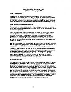
GA - Multi Variable Unconstrained Test Function: 3 Function 3:
10×2+(x2-10 cos(2πx))+(y2-10 cos(2πy)), minimum at f(0,0)=0, for -5.12≤ (x,y) ≤ 5.12. f(x,y)=20+(x2-10cos(2*pi()*x))+(y2-10cos(2*pi()*y))
f(x,y)
GA Parameters: 100 Resolution: 10-10 80 Population size: 200 Cross-over rate: 40% of population 60 Generations: 100 40 20 0 5 5 0
y
0 -5
-5
x Dr. K. Shankar
MDS, IIT Madras, Chennai-36.
GA-MATLAB code for Function 3 %% FILE: GA_Optimization_Two_Variables_3.m % *********************************************************************** % A MATLAB Program to optimize the given test function of multi variable % using genetic algorithm toolbox with options ‘ga’ % *********************************************************************** %% clear all; close all; clc; format shortg; % Clearing the screen % *********************************************************************** % PLOT THE GIVEN FUNCTION % *********************************************************************** x=-5:0.1:5; % Variable x bounds (-5,5) y=-5:0.1:5; % Variable y bounds (-5,5) [X Y]=meshgrid(x,y); % Generate X and Y arrays for 3-D plots fxy=10*2+(X.^2-10*cos(2*pi()*X))+(Y.^2-10*cos(2*pi()*Y));% Test function f(x,y) surfc(X,Y,fxy); % Plot the function surface title('f(x,y)=20+(x^2-10cos(2*pi()*x))+(y^2-10cos(2*pi()*y))');% Title of the plot xlabel('x'); ylabel('y'); zlabel('f(x,y)'); % Labels of x, y and z % *********************************************************************** % FUNCTION OPTIMIZATION BY GENETIC ALGORITHM (GA) % *********************************************************************** options=optimset(@ga); % Default GA options options.TolFun=1e-10; % Resolution options.Generations=100; % Number of generations options.PopulationSize=200; % Population size options.CrossoverFraction=0.4; % Cross-over faction options.PlotFcns=@gaplotbestf; % Ploting function as best fitness options.Display='iter'; % Iteration display fun=@(x)(2*10+(x(1)^2-10*cos(2*pi()*x(1)))+...% . (x(2)^2-10*cos(2*pi()*x(2)))); % function to be optimized nvars=2; % Number of variables A=[]; b=[]; % Linear inequality constraints Aeq=[];beq=[]; % Equality constraints xl=[0 0]; xu=[10 10]; % Lower and upper bounds nonlcon=[]; % Non-linearity constraints [x,fval]=ga(fun,nvars,A,b,Aeq,beq,xl,xu,nonlcon,options);% Optimization command disp('x*'); disp(x); % x*: Optimal x disp('f(x*)'); disp(fval); % function value at x*
Dr. K. Shankar
MDS, IIT Madras, Chennai-36.
GA-MATLAB output for Function 3
Best: 0 Mean: 1.4962e-006 Best fitness Mean fitness
Fitness value
% *********************************************************************** % GA OPTIMIZATION OUTPUT % *********************************************************************** % Best Mean Stall % Generation f-count f(x) f(x) Generations % 1 400 0 15.59 0 % 2 600 0 11.22 1 % 3 800 0 15.96 2 20 % 4 1000 0 12.89 3 % 5 1200 0 9.201 4 18 % 6 1400 0 5.85 5 16 % 7 1600 0 3.424 6 14 % 8 1800 0 1.839 7 % 9 2000 0 1.004 8 12 % 10 2200 0 0.4435 9 10 % 20 4200 0 1.793e-006 19 % 30 6200 0 2.349e-006 29 8 % 40 8200 0 1.501e-006 39 6 % 41 8400 0 1.449e-006 40 4 % 42 8600 0 1.52e-006 41 % 43 8800 0 1.616e-006 42 2 % 44 9000 0 1.685e-006 43 0 % 45 9200 0 1.594e-006 44 0 10 % 46 9400 0 1.667e-006 45 % 47 9600 0 1.606e-006 46 % 48 9800 0 1.797e-006 47 % 49 10000 0 1.849e-006 48 % 50 10200 0 1.821e-006 49 % 51 10400 0 1.496e-006 50 % Optimization terminated: average change in the fitness value less than options.TolFun. % x* % 0 0 % % f(x*) % 0
20
30
40
50 60 Generation
70
80
90
Dr. K. Shankar MDS, IIT Madras, Chennai-36.
100