Memoirs of the Faculty of Engineering, Okayama University, Vol. 44, pp. 32–41, January 2010
Optimization without Search: Constraint Satisfaction by Orthogonal Projection with Applications to Multiview Triangulation Kenichi KANATANI∗, Hirotaka NIITSUMA Department of Computer Science Okayama University Okayama 700-8530 Japan
Yasuyuki SUGAYA Department of Information and Computer Sciences Toyohashi University of Technology Toyohashi, Aichi 441-8580 Japan
(Received December 24, 2009)
We present an alternative approach to what we call the “standard optimization”, which minimizes a cost function by searching a parameter space. Instead, the input is “orthogonally projected” in the joint input space onto the manifold defined by the “consistency constraint”, which demands that any minimal subset of observations produce the same result. This approach avoids many difficulties encountered in the standard optimization. As typical examples, we apply it to line fitting and multiview triangulation. The latter produces a new algorithm far more efficient than existing methods. We also discuss optimality of our approach.
estimation is based on the knowledge that the data xκ should ideally satisfy some constraint parameterized by θ. However, it is violated in the presence of noise. Let E(θ; x0 , ..., xM −1 ) measure the cost (also called “energy”) of this violation. We compute the value of θ that minimizes E. A widely adopted cost is defined by expressing the ideal value of xκ , given ¯ κ (θ) and minimizing θ, in the form x
1. INTRODUCTION For extracting a geometric structure from noisy images, numerical optimization is vital. A widely accepted approach is the standard optimization, minimizing a cost function by searching a parameter space. In this paper, we present an alternative approach of orthogonally projecting the input onto the manifold in the joint input space defined by the consistency constraint, which demands that any minimal subset of observations produce the same result. We show how this approach avoids many difficulties encountered in the standard optimization. We first describe the standard optimization in Sec. 2 and summarize existing global optimization techniques in Sec. 3. We describe our orthogonal projection approach in Sec. 4 and apply it to line fitting in Sec. 5. Then, we apply our approach to multiview triangulation in Sec. 6 and demonstrate by experiments in Sec. 7 that the resulting algorithm is far more efficient than existing methods. In Sec. 8, we conclude and discuss optimality of our approach.
E=
(1)
This includes what is known as bundle adjustment, where Eq. (1) is called the reprojection error. 3. GLOBAL OPTIMIZATION The major problem of the standard optimization as defined above is the difficulty of finding an absolute minimum of the cost E. The parameter space of θ is usually infinitely large and high-dimensional. Well known search techniques include Newton iterations and conjugate gradient search. For bundle adjustment, the Leverberg-Marquardt method is the standard tool. However, such gradient-based search may fall into local minima. In recent years, intensive efforts have been made to minimize E globally [1].
Given M observations xκ , κ = 0, ..., M − 1, we want to estimate a parameter θ that specifies the structure that should exist in the input images. The
Algebraic methods. We let the derivatives of E with respect to the parameters be zero, compute
[email protected]
——————— This work is subjected to copyright. All rights are reserved by this author/authors.
k¯ xκ (θ) − xκ k2 .
κ=0
2. STANDARD OPTIMIZATION
∗ E-mail
M −1 ∑
32
Kenichi KANATANI et al.
MEM.FAC.ENG.OKA.UNI. Vol. 44
all solutions exhaustively, and choose the one for which E is the smallest. In many vision applications, we obtain a set of algebraic equations, which reduces, via the Gr¨ obner basis, to a single polynomial. However, its degree is usually very high, and numerical evaluation is unstable and inefficient.
1. If there were no noise, the parameter θ could immediately be computed. In fact, algebraic procedures have been intensively studied for computing geometric properties from exact image data [4]. 2. There exists a minimum number of (nondegenerate) observations (call it a minimal set) that can uniquely determine the value of θ. For example, a line is uniquely determined by two points, an ellipse by four points, and a fundamental matrix by seven pairs of corresponding points.
Branch and bound. Introducing a function that gives a lower bound of E locally, we partition the parameter space into small cells, evaluating a representative value and a lower bound in each cell. Those cells for which the lower bound is larger than the values already evaluated in other cells are discarded; the remaining cells are recursively subdivided. However, the lower bounding process is often complicated, requiring a large amount of computation.
3. Given redundant observations, we can choose from among them any minimal set for determining θ. In the presence of noise, however, the solution depends on which minimal set is chosen. The standard optimization overcomes this dependence on the choice of the minimal set by minimizing a cost E over the parameter space of θ. Our alternative does not introduce any cost but minimally corˆ 0 , ..., x ˆ M −1 rects the observations x0 , ..., xM −1 into x to enforce the condition, which we call the consistency constraint, that any choice of the minimal set result in the same solution. Once this constraint is satisfied, we can choose any minimal set to determine θ. By minimally, we mean that the correction is done in such a way that
Matrix inequality optimization. Changing variables, we reduce the problem to polynomial minimization subject to matrix inequalities [7]. This has the form of SDP (semidefinite program), which can be solved by a Matlab tool called GloptiPoly. The resulting solution is approximate, but it is theoretically proved to approach the true solution as the number of variables and the size of the accompanying matrices are increased. A complicate analysis and a large amount of computation are necessary if we want to reach a high accuracy.
E=
M −1 ∑
kˆ xκ − xκ k2 ,
(2)
κ=0
L∞ optimization. Minimizing Eq. (1) is regarded as maximum likelihood (ML) if the noise is independent and identical Gaussian, which is appropriate in many applications. However, this makes global optimization difficult, so we replace the L2 norm in Eq. (1) by L∞ [2, 5, 9]. Then, the cost E usually becomes quasi-convex. We gradually increase the threshold from 0 (or using binary search) and check if there exists a value of E above the threshold. This problem usually has the form of SOCP (second-order cone program), which can be solved by a Matlab tool called SeDuMi.
which we call the reprojection error , is the smallest. Evidently, the solution is the same as the standard optimization using the cost of Eq. (1). Our approach can be geometrically interpreted as follows. Let F (x0 , ..., xM −1 ) = 0,
(3)
be the consistency constraint, which may be a set of equations. This defines a manifold S in the joint space of x0 , ..., xM −1 . Our goal is to find a point pˆ ˆ0 ⊕ · · · ⊕ x ˆ M −1 ∈ S closest to the observation p =x = x0 ⊕ · · · ⊕ xM −1 ; the square distance |pˆ p|2 is the reprojection error in Eq. (2). Thus, the solution is obtained by orthogonally projecting p onto S (Fig. 1). The standard optimization using Eq. (1) can be interpreted as follows. Introducing the parameter θ is equivalent to parameterizing S. We search the inside of S to find a location (i.e., its “coordinates” θ) closest to p. Gradient-based search may fall into local minima, but finding a global minimum is difficult, as described earlier.
All these approaches need a complicated analysis and a large amount of computation, requiring various optimization tools, whose performance is not always guaranteed. 4. ORTHOGONAL PROJECTION We now present a complementary approach: we do not search the parameter space; we do not minimize any function. We directly reach an optimal solution by imposing constraints on the data. Our approach is motivated by the following observations:
5. LINE FITTING We now apply our approach to a simplest example: fitting a line to points. Although this does not 33
January 2010
Optimization without Search: Constraint Satisfaction by Orthogonal Projection
Eq. (7), onto S. Note that we neither introduce any parameterization to the line to be fitted nor define any cost function to minimize. ˆ0 ⊕ · · · ⊕ x ˆ M −1 be the desired projection, Let pˆ = x ˆ κ = xκ − ∆xκ . Substituting x ˆ κ into Eq. (7) and let x and expanding it to a first order in ∆xκ , we obtain
S p=x0 +
+ xM-1 E initial
E min p=x 0 +
E local min + xM-1
(∆xκ , xκ+1 × xκ+2 ) + (∆xκ+1 , xκ+2 × xκ ) +(∆xκ+2 , xκ × xκ+1 ) = |xκ , xκ+1 , xκ+2 |, (8)
Figure 1: Orthogonal projection of p = x0 ⊕ · · · ⊕ xM −1
where and throughout this paper we denote by (a, b) the inner product of a and b. Since Eq. (8) is linear in ∆xκ , the M − 2 equations in this form, when viewed ˆ κ through ∆xκ = xκ − as equations of free variables x ˆ κ , define a plane2 Π that approximates the manifold x S. We now compute a projection direction ∆x0 ⊕· · ·⊕ ∆xM −1 orthogonal to Π. This is obtained in the form
onto the manifold S gives the minimum reprojection error Emin . The standard optimization starts from some point in S and searches the “inside” of S, where the consistency constraint is always satisfied, but may stop at a local minimum Elocal min .
produce practical benefits, since the problem is immediately solved by the standard optimization, this will illustrate how our approach works. Given M points (x0 , y0 ), ..., (xM −1 , yM −1 ), the standard optimization goes like this. We first parameterize the line, say Ax + By + C = 0, the parameter being θ = (A, B, C)> . The distance dκ of point (xκ , yκ ) from this line is dκ =
|Axκ + Byκ + C| √ . A2 + B 2
∆xκ = λκ P k (xκ+1×xκ+2 )+λκ−1 P k (xκ+1×xκ−1 ) +λκ−2 P k (xκ−2 × xκ−1 ),
(9)
where λκ are unknown parameters and P k ≡ diag(1, 1, 0) and (see Appendix A.1 for the derivation). We adjust the parameters λκ so that the projection reaches the plane Π. Substitution of Eq. (9) into Eq. (8) results in simultaneous linear equations in λκ in the form
(4)
We minimize the sum of square distances: E(A, B, C) =
M −1 ∑ κ=0
Aκ λκ−2+Bκ λκ−1+Cκ λκ+Dκ λκ+1+Eκ λκ+2 = Fκ , (10) (Axκ + Byκ + C)2 . A2 + B 2
(5)
where Aκ = (P k (xκ−2 × xκ−1 ), P k (xκ+1 × xκ+2 )), Bκ = (P k (xκ+1 × xκ−1 ), P k (xκ+1 × xκ+2 ))
The solution is analytically obtained by solving a 2×2 eigenvalue problem. Our approach is different. We represent the point (xκ , yκ ) by the 3-D vector xκ /f0 xκ = yκ /f0 , (6) 1
+(P k (xκ−1 × xκ ), P k (xκ+2 × xκ )), Cκ = kP k (xκ+1 × xκ+2 )k2 + kP k (xκ+2 × xκ )k2 +kP k (xκ × xκ+1 )k2 , Dκ = (P k (xκ+2 × xκ+3 ), P k (xκ+2 × xκ )) +(P k (xκ+3 × xκ+1 ), P k (xκ × xκ+1 )),
where f0 is a scale normalization constant of approximately the image size1 . Three points xκ , xλ , and xµ are collinear if and only if their scalar triple product |xκ , xλ , xµ | is zero. Hence, the consistency (or collinearity in this case) constraint is |xκ , xκ+1 , xκ+2 | = 0,
Eκ = (P k (xκ+3 × xκ+4 ), P k (xκ × xκ+1 )), Fκ = |xκ , xκ+1 , xκ+2 |.
(11)
Solving Eq. (10) and substituting the resulting λκ ˆ κ = xκ − ∆xκ . The into Eq. (9), we can determine x ˆ 0 ⊕· · ·⊕ x ˆ M −1 is orthogonal resulting projection pˆ = x to the plane Π by construction but not necessarily to ˆˆ 0 ⊕ · · · ⊕ x ˆˆ M −1 so ˆˆ = x S itself. So, we correct pˆ to p ˆ ˆ ˆκ = x ˆ κ − ∆xˆκ , we substitute that pˆ ∈ S. Letting x ˆˆ κ for xκ in Eq. (7). The first order expansion at x ˆκ x in the higher order term ∆ˆ xκ is
(7)
for κ = 0, ..., M − 3. These M − 2 equations define an (M + 2)-D manifold S in the 2M -D joint space of (x0 , y0 , ... xM −1 , yM −1 ). The dimension of S corresponds to the two degrees of freedom of the line to be fitted and the positions of the M points on it. We now orthogonally project the observation p = x0 ⊕ · · · ⊕ xM −1 , which does not necessarily satisfy
ˆ κ+1 × x ˆ κ+2 ) + (∆ˆ ˆ κ+2 × x ˆ κ) (∆ˆ xκ , x xκ+1 , x ˆκ × x ˆ κ+1 ) = |ˆ ˆ κ+1 , x ˆ κ+2 |. +(∆ˆ xκ+2 , x xκ , x
1 This
is merely for making the three components to have the same order of magnitude for numerical stability. Theoretically, it can be set to any value, e.g., 1.
2 Strictly
(12)
speaking, this is an (M + 2)-D affine space, but we call this a “plane” for short.
34
Kenichi KANATANI et al.
MEM.FAC.ENG.OKA.UNI. Vol. 44
ˆ κ , κ = 0, ..., M − 1, Output: Corrected positions x and the reprojection error E.
p Π
Procedure:
p
Π
ˆ κ = xκ , x ˜ κ = 0, κ = 0, ..., M − 1, 1. Let E0 = ∞, x where ∞ is a sufficiently large number.
∆p S
p
2. Compute Aκ , ..., Fκ , κ = 0, ..., M − 3, by Eqs. (14).
Figure 2: Successive orthogonal projection onto S. The
3. Solve the following set of linear equations in λκ , κ = 0, ..., M − 3:
orthogonal projection from p to Π minimizes kp − pˆk2 , ˆ minimizes while the orthogonal projection from p to Π 2 2 ˆ kp− pˆk = kp− pˆ+∆ˆ pk , where ∆ˆ p = ∆ˆ x0 ⊕· · ·⊕∆ˆ xM −1 .
λ0 C0 D0 E0 λ1 B1 C1 D1 E1 λ2 A2 B2 C2 D2 E2 λ3 A3 B3 C3 D3 E3 .. .. .. .. .. . . . . . λM −3 AM −3 BM −3 CM −3 F0 F1 F2 = F3 . (16) .. . FM −3
ˆ that The M −2 equations in this form define a plane Π approximates S better than Π. We compute a new orthogonal projection to it. Note that the projection always starts from the observation p = x0 ⊕· · ·⊕xM −1 , not from pˆ (Fig. 2). The new projection direction is given by ˆ κ+2 )+λκ−1 P k (ˆ ˆ κ−1 ) ∆ˆ xκ = λκ P k (ˆ xκ+1× x xκ+1× x ˆ κ−1 ) − x ˜ κ, +λκ−2 P k (ˆ xκ−2 × x (13) where we define ˜ κ = xκ − x ˆ κ. x
(14)
(See Appendix A.2 for the derivation.) The parameters λκ are determined so that that the projection ˆ Substitution of Eq. (13) into reaches the plane Π. Eq. (12) results in simultaneous linear equations in λκ in the same form as Eq. (10) except that Aκ , ..., Fκ are now replaced by
˜ κ and x ˆ κ , κ = 0, ..., M − 1, as follows: 4. Update x ˜ κ ← λκ P k (ˆ ˆ κ+2 )+λκ−1 P k (ˆ ˆ κ−1 ) x xκ+1× x xκ+1× x ˆ κ−1 ), +λκ−2 P k (ˆ xκ−2× x ˆ κ ← xκ − x ˜ κ. x (17)
ˆ κ−1 ), P k (ˆ ˆ κ+2 )), Aκ = (P k (ˆ xκ−2 × x xκ+1 × x ˆ κ−1 ), P k (ˆ ˆ κ+2 )) Bκ = (P k (ˆ xκ+1 × x xκ+1 × x ˆ κ ), P k (ˆ ˆ κ )), +(P k (ˆ xκ−1 × x xκ+2 × x 2 ˆ κ+2 )k + kP k (ˆ ˆ κ )k2 Cκ = kP k (ˆ xκ+1 × x xκ+2 × x 2 ˆ κ+1 )k , +kP k (ˆ xκ × x
5. Compute the reprojection error E as follows: E=
ˆ κ+3 ), P k (ˆ ˆ κ )) Dκ = (P k (ˆ xκ+2 × x xκ+2 × x ˆ κ+1 ), P k (ˆ ˆ κ+1 )), +(P k (ˆ xκ+3 × x xκ × x ˆ κ+4 ), P k (ˆ ˆ κ+1 )), Eκ = (P k (ˆ xκ+3 × x xκ × x ˆ κ+1 , x ˆ κ+2 | + |˜ ˆ κ+1 , x ˆ κ+2 | Fκ = |ˆ xκ , x xκ , x ˜ κ+1 , x ˆ κ+2 | + |ˆ ˆ κ+1 , x ˜ κ+2 |. +|ˆ xκ , x xκ , x
M −1 ∑
k˜ xκ k2 .
(18)
κ=0
ˆ κ , κ = 0, ..., 6. If |E − E0 | ≈ 0, return E and x M − 1, and stop. Else, let E0 ← E, and go back to Step 2.
(15)
Once we have imposed the consistency constraint, we can pick out any two (distinct) points and compute the line connecting them.
Solving Eq. (10) and substituting the resulting λκ in ˆ ˆ κ = xκ − ∆ˆ Eq. (13), we can determine x xκ . The reˆ by construction sulting projection is orthogonal to Π but still may not be orthogonal to S itself. So, we let ˆˆ κ and repeat this correction. In the end, ∆ˆ ˆκ ← x x xκ ˆˆ ∈ S. Because the plane Π ˆ is a first = 0 and pˆ = p order expansion of S at pˆ ∈ S, it is tangent to S at ˆ it is orthogonal to S pˆ. Since pˆ p is orthogonal to Π, itself. Our algorithm is summarized as follows:
6.
TRIANGULATION FROM MULTIPLE VIEWS
The above line fitting algorithm does not produce practical benefits, but we can derive, using the same principle, a new algorithm for triangulation from multiple views.
Input: Data points xκ , κ = 0, ..., M − 1. 35
January 2010
Optimization without Search: Constraint Satisfaction by Orthogonal Projection
where λpq (κ) are unknown parameters (Appendix A.3 for the derivation). Here, we define
6.1 Problem Suppose we have M cameras. We assume that their intrinsic and extrinsic parameters are known. Let (xκ , yκ ) be the image of a 3-D point (X, Y, Z) in the κth view. Our task is to compute (X, Y, Z) from (xκ , yκ ), κ = 0, ..., M − 1. If (xκ , yκ ) are exact, we can pick out any two (nondegenerate) views and compute (X, Y, Z) by elementary triangulation. If (xκ , yκ ) are not exact, however, the rays, call them the lines of sight, starting from the projection centers and passing through the points in the images, do not meet at a single point in the scene. Traditionally, this has been dealt with by the standard optimization [1]: we search the 3-D space for θ = (X, Y, Z)> that minimizes the reprojection error of Eq. (1). Our approach is as follows. As line fitting, we represent each point (xκ , yκ ) by the 3-D vector in Eq. (6). The consistency constraint we adopt is lm i ²ljp ²mkq T(κ)i x(κ) xj(κ+1) xk(κ+2)
= 0,
s lm P(κ)pq = ²ljp ²mkq T(κ)i Pksi xjκ+1 xkκ+2 , lm xiκ−1 Pksj xkκ+1 , Qs(κ)pq = ²ljp ²mkq T(κ−1)i s lm R(κ)pq = ²ljp ²mkq T(κ−2)i xiκ−2 xjκ−1 Pksk .
(22)
The symbol Pkij denotes the (ij) element of the matrix P k (= diag(1, 1, 0)). We adjust the parameters λpq (κ) ˆ0 ⊕ · · · ⊕ x ˆ M −1 be on all so that the projection pˆ = x the hyperplanes in Π. Such a solution may not exist, but we proceed as if there is. Substituting Eq. (21) into Eq. (20), we obtain rs rs A(κ)pqrs λrs (κ−2) + B(κ)pqrs λ(κ−1) + C(κ)pqrs λ(κ) rs +D(κ)pqrs λrs (23) (κ+1) + E(κ)pqrs λ(κ+2) = F(κ)pq ,
where we define
(19)
lm i R(κ)rs xjκ+1 xkκ+2 , A(κ)pqrs = ²ljp ²mkq T(κ)i ( lm Qi(κ)rs xjκ+1 xkκ+2 B(κ)pqrs = ²ljp ²mkq T(κ)i ) j + xiκ R(κ+1)rs xkκ+2 , ( lm i xjκ+1 xkκ+2 C(κ)pqrs = ²ljp ²mkq T(κ)i P(κ)rs
for κ = 0, ..., M − 3, where is the trifocal tensor for the κth, the (κ + 1)st, and the (κ + 2)nd views; ²ijk is the permutation symbol. We use Einstein’s convention for omitting the summation symbol over repeated upper and lower indices. Equation (19) is known as the trilinear constraint, which provides a necessary and sufficient condition that the lines of sight from the three cameras meet at a single point in the scene [4]. The M − 2 equations in Eq. (19) guarantee that the M lines of sight have a common intersection. The M − 2 equations in Eq. (19) define a manifold S in the joint 2M -D space of (x0 , y0 , ..., xM −1 , yM −1 ). Our task is to orthogonally project the observation p ˆ0 ⊕ · · · ⊕ x ˆ M −1 = x0 ⊕ · · · ⊕ xM −1 onto S. Let pˆ = x ˆ κ = xκ − ∆xκ . be the desired projection, and let x ˆ κ and expanding it to a Replacing xκ in Eq. (19) by x first order in ∆xκ , we obtain (the summation symbol is omitted by Einstein’s convention) ( ) lm ²ljp ²mkq T(κ)i ∆xiκ xjκ+1 xkκ+2 + xiκ ∆xjκ+1 xkκ+2 lm T(κ)i
j + xiκ R(κ+1)rs xkκ+2 + xiκ Qj(κ+1)rs xkκ+2
) j k + xiκ R(κ+1)rs xkκ+2 + xiκ xjκ+1 R(κ+2)rs , ( j lm D(κ)pqrs = ²ljp ²mkq T(κ)i xiκ P(κ+1)rs xkκ+2 ) j xkκ+2 + xiκ xjκ+1 Qk(κ+2)rs , + xiκ R(κ+1)rs lm i j k E(κ)pqrs = ²ljp ²mkq T(κ)i xκ xκ+1 P(κ+2)rs , lm i j F(κ)pq = ²ljp ²mkq T(κ)i xκ xκ+1 xkκ+2 .
(24)
Equation (23) provides 9(M −2) linear equations (r, s = 1, 2, 3, κ = 0, ..., M − 3) in the 9(M − 2) unknowns λpq (κ) (p, q = 1, 2, 3, κ = 0, ..., M − 3). However, Eq. (23) is derived on the assumption that there is a solution, but it has a unique solution only when p = x0 ⊕ · · · ⊕ xM −1 ∈ S; the solvability condition is gradually violated as p departs from S. We discuss how to cope with this shortly. Once λpq (κ) is obtained, ˆκ we can determine ∆xκ by Eq. (21) and compute x = xκ − ∆xκ . Now, we go the second round. Replacing xκ in ˆˆ κ = x ˆ κ − ∆ˆ Eq. (19) by x xκ and expanding it to a first order in ∆ˆ xκ , we obtain ( lm ²ljp ²mkq T(κ)i ∆ˆ xiκ x ˆjκ+1 x ˆkκ+2 + x ˆiκ ∆ˆ xjκ+1 x ˆkκ+2 ) lm i j +ˆ xiκ x ˆjκ+1 ∆ˆ xkκ+2 = ²ljp ²mkq T(κ)i x ˆκ x ˆκ+1 x ˆkκ+2 , (25)
lm i j +xiκ xjκ+1 ∆xkκ+2 = ²ljp ²mkq T(κ)i xκ xκ+1 xkκ+2 . (20)
The resulting 9(M − 2) equations for p, q = 1, 2, 3 and κ = 0, ..., M −3, when viewed as equations of free ˆ κ through ∆xκ = xκ − x ˆ κ , define a set Π variables x of 9(M − 2) hyperplanes in 2M -D that approximate S. They would intersect at a 3-D affine space if p = x0 ⊕ · · · ⊕ xM −1 ∈ S. Otherwise, they may not have a common intersection. We now determine a projection direction ∆x0 ⊕ · · · ⊕ ∆xM −1 orthogonal to all the hyperplanes in Π. Such a direction may not exist, but we proceed as if there is; the nonexistence condition emerges later. If there are such ∆xκ , they should have form
ˆ of hyperplanes that should which defines a set Π approximate S better than those in Π, since pˆ =
pq pq i i i ∆xsκ = P(κ)pq λpq (κ) +Q(κ)pq λ(κ−1) +R(κ)pq λ(κ−2) , (21)
36
Kenichi KANATANI et al.
MEM.FAC.ENG.OKA.UNI. Vol. 44
ˆ0 ⊕ · · · ⊕ x ˆ M −1 is expected to be closer to S than x ˆ would p = x0 ⊕ · · · ⊕ xM −1 . The hyperplanes in Π intersect at a 3-D affine space if pˆ ∈ S. We determine a new projection direction ∆ˆ x0 ⊕ · · · ⊕ ∆ˆ xM −1 orˆ although such a thogonal to all the hyperplanes in Π, direction may not exist. If there are such ∆xκ , they should have the form ∆ˆ xsκ =
3 ∑
s Pˆ(κ)pq λpq (κ) +
p,q=1
+
3 ∑
at pˆ ∈ S, they are tangent to S at pˆ, defining the tangent space Tpˆ(S) at pˆ as their intersection. Since ˆ it pˆ p is now orthogonal to all the hyperplanes in Π, is orthogonal to S itself. 6.2 Rank deficiency There is one added complexity due to the fact that Eq. (19) has redundancies: each trilinear constraint consists of nine equalities for p, q = 1, 2, 3, and only four are linearly independent due to the skew properties of ²ijk . Hence, Eq. (19) consists of 9(M − 2) equalities, 4(M −2) of which are linearly independent. Among them, however, only 2M − 3 are algebraically independent. This is because the manifold S should be homeomorphic to R3 , since a point in S is in oneto-one correspondence to a point to be reconstructed in R3 as the unique intersection of the lines of sight. Thus, S is 3-D and can be defined as an intersection of 2M − 3 hypersurfaces; the remaining hypersurfaces automatically pass through it. We enumerate the index pairs (p, q) = (1,1), (1,2), ..., (3,3) with a serial number α = 1, ..., 9 and (r, s) = (1,1), (1,2), ..., (3,3) with β = 1, ..., 9, and identify ˆ(κ)pqrs , etc. with 9 × 9 matrices. Likewise, Aˆ(κ)pqrs , B ˆ Fˆ(κ)pq and λpq (κ) are identified with 9-D vectors f (κ) and λ(κ) , respectively. Then, Eq. (23) now takes the form C 0 D0 E 0 λ0 B 1 C 1 D1 E 1 λ1 A2 B 2 C 2 D 2 λ2 E2 .. .. .. .. . . . .
pq ˆs Q (κ)pq λ(κ−1)
p,q=1
3 ∑
pq ˆs R ˜iκ , (κ)pq λ(κ−2) − x
(26)
p,q=1
where we define ˜ κ = xκ − x ˆ κ, x
(27)
and s lm Pˆ(κ)pq = ²ljp ²mkq T(κ)i Pksi x ˆjκ+1 x ˆkκ+2 , lm ˆs ˆkκ+1 , Q ˆiκ−1 Pksj x (κ)pq = ²ljp ²mkq T(κ−1)i x lm ˆs R ˆiκ−2 x ˆjκ−1 Pksk . (κ)pq = ²ljp ²mkq T(κ−2)i x
(28)
(See Appendix A.4 for the derivation.) We adjust the parameters λpq (κ) so that the resulting projection be ˆ although such a solution on all the hyperplanes in Π, may not exist. Substituting Eq. (26) into Eq. (25), we obtain simultaneous linear equations in λpq (κ) in the same form as Eq. (23) except that A(κ)pqrs , ..., F(κ)pq are now replaced by lm ˆ i ˆkκ+2 , R(κ)rs x ˆjκ+1 x A(κ)pqrs = ²ljp ²mkq T(κ)i ( lm ˆi B(κ)pqrs = ²ljp ²mkq T(κ)i Q ˆjκ+1 x ˆkκ+2 (κ)rs x ) k ˆj +x ˆiκ R x ˆ (κ+1)rs κ+2 , ( lm i ˆkκ+2 C(κ)pqrs = ²ljp ²mkq T(κ)i Pˆ(κ)rs x ˆjκ+1 x
f0 f1 = f2 , .. . f M −3
ˆj ˆkκ+2 +x ˆiκ Q (κ+1)rs x ) ˆk +ˆ xiκ x ˆjκ+1 R (κ+2)rs ,
λM −3
(30)
where Aκ , ..., E κ are 9 × 9 matrices, and λκ and f κ are 9-D vectors. The coefficient matrix has a band of width 45. Eq. (30) may not necessarily have a ˆ0 ⊕ · · · ⊕ x ˆ M −1 ∈ S. The unique solution unless pˆ = x 9(M − 2) × 9(M − 2) coefficient matrix generally has rank 2M , because the underlying unknowns are 2M variables ∆x0 , ∆y0 , ..., ∆xM −1 , ∆yM −1 . However, the rank drops to 2M −3 at the moment the projection ˆ0 ⊕ · · · ⊕ x ˆ M −1 reaches S, which is our goal. pˆ = x Hence, we select appropriate 2M − 3 equations from among the 9(M − 2) equations in Eq. (30), which is mathematically equivalent to using the pseudoinverse of rank 2M − 3. Our algorithm is summarized as follows:
( j lm D(κ)pqrs = ²ljp ²mkq T(κ)i x ˆiκ Pˆ(κ+1)rs x ˆkκ+2 ) ˆk +x ˆiκ x ˆjκ+1 Q (κ+2)rs , lm i j k E(κ)pqrs = ²ljp ²mkq T(κ)i x ˆκ x ˆκ+1 Pˆ(κ+2)rs , ( lm F(κ)pq = ²ljp ²mkq T(κ)i x ˆiκ x ˆjκ+1 x ˆkκ+2
) +x ˜iκ x ˆjκ+1 x ˆkκ+2 + x ˆiκ x ˜jκ+1 x ˆkκ+2 + x ˆiκ x ˆjκ+1 x ˜kκ+2 .
AM −3 B M −3 C M −3
(29)
Solving Eqs. (23) and substituting the resulting λpq (κ) ˆˆ κ in Eq. (26), we can determine ∆ˆ xκ and compute x ˆ κ , we repeat this proceˆ κ − ∆ˆ ˆκ ← x ˆ =x xκ . Letting x ˆˆ ∈ S. Because dure. In the end, ∆ˆ xκ = 0 and pˆ = p ˆ are first order expansions of S the hyperplanes in Π
Input: Data points xκ , κ = 0, ..., M − 1, and the jk trifocal tensors T(κ)i , κ = 0, ..., M − 2. 37
January 2010
Optimization without Search: Constraint Satisfaction by Orthogonal Projection
ˆ κ , κ = 0, ..., M − 1, Output: Corrected positions x and the reprojection error E. ···
Procedure:
···
ˆ κ = xκ , x ˜ κ = 0, κ = 0, ..., M − 1, 1. Let E0 = ∞, x where ∞ is a sufficiently large number. s s ˆ spq , and R ˆ pq 2. Compute Pˆpq ,Q in Eqs. (28).
Figure 3: Simulated images of a cylindrical grid surface.
3. Compute Apqrs , ..., Fpq in Eqs. (29). 4. Solve Eq. (30) for rank 2M − 3.
λpq (κ) ,
-3
x10
using pseudoinverse of
200
3
150 2
100
˜ κ and x ˆ κ , κ = 0, ..., M − 1, as follows: 5. Update x 1
x ˜iκ ←
3 ∑
i P(κ)pq λpq (κ) +
p,q=1
+
3 ∑
Qi(κ)pq λpq (κ−1)
0
i R(κ)pq λpq (κ−2o) ,
M −1 ∑
k˜ xκ k2 .
8
σ
10
0
2
4
6
8
σ
(b)
7. EXPERIMENTS 7.1 Accuracy
(32)
κ=0
We created synthetic images of a cylindrical grid surface viewed by cameras surrounding it. Fig. 3 shows some of them. The image size is 1000 × 1000 pixels, and the focal length is f = 600 pixels. Independent Gaussian noise of mean 0 and standard deviation σ pixels is added to the x and the y coordinates of each grid point, and our algorithm3 is applied. We stopped when the update of the reprojection error E is less than 10−6 . The solid line in Fig. 4(a) shows the average reprojection error per point over 1000 trials for each σ. The dashed line is the corresponding result of least squares (the linear method). The dotted line shows the first order theoretical expectation (2M − 3)(σ/f0 )2 for maximum likelihood (ML); we can see that the ML solution is indeed computed by our method. The solid line in Fig. 4(b) shows the average RMS error per point of the reconstructed 3-D position. We see that although the reprojection error is not much different between least squares and our method, the 3-D reconstruction accuracy is markedly distinct between them.
ˆ κ , κ = 0, ..., 7. If |E − E0 | ≈ 0, return E and x M − 1, and stop. Else, let E0 ← E, and go back to Step 2. 6.3 Efficient computation We frequently encounter expressions in the form Tpq = ²ljp ²mkq Tilm xi y j z k ,
6
of 3-D. Solid lines: our method. Dashed lines: least squares. Dotted lines: theoretical expectation (2M − 3)(σ/f0 )2 .
(31)
6. Compute the reprojection error E as follows:
E=
4
Figure 4: (a) Average reprojection error. (b) RMS error
p,q=1
ˆ κ ← xκ − x ˜ κ. x
2
(a)
p,q=1
3 ∑
50
(33)
lm where Tilm takes Ti(κ) , and xi , y j , and z k take, respecˆ κ , or x ˜ κ . The tively, the i, j, k components of xκ , x right-hand side of Eq. (33) is a sum over i, j, k, l, m = 1, 2, 3 (the summation symbol omitted), so we need to add 35 = 243 terms. These summations cost a considerable computation time. It can be significantly reduced if we note that Eq. (33) can be equivalently rewritten as ( Tpq = xi Tip⊕1,q⊕1 y p⊕2 z q⊕2 −Tip⊕2,q⊕1 y p⊕1 z q⊕2 ) − Tip⊕1,q⊕2 y p⊕2 z q⊕1 +Tip⊕2,q⊕2 y p⊕1 z q⊕1 , (34)
7.2 Computation time Fig. 5 shows the average computation time per point (average over 10 trials) for M = 3, 4, ..., 31 views with noise of σ = 5 pixels. We used C++ with
where ⊕ denotes addition modulo 3. The right-hand side is a sum over i = 1, 2, 3, so we need to add only 3 × 4 = 12 terms. This makes the computation about 243/12 (≈ 20) times more efficient.
3 http://www.iim.ics.tut.ac.jp/~sugaya/public.php
38
10
Kenichi KANATANI et al.
0.3
MEM.FAC.ENG.OKA.UNI. Vol. 44
of Kahl et al. [6] took 5030 sec, i.e., 1.01 sec per point. Lu and Hartley [10] reported that their C++ program of branch and bound applied for a different data set took 0.02 sec per point. Fair and definitive comparison is difficult; existing methods all use complicated algorithms involving black box software tools and are difficult to implement from scratch. Also, the codes offered by the authors are written in different environments. Still, the above observations suggest that our algorithm is far faster than all existing standard optimization methods.
sec
0.2
0.1
0
5
10
15
20
25
Μ 30
Figure 5: Computation time (sec) vs. the number M of views. The dotted line aM e is fitted with a = 4.17 × 10⁻⁶ and e = 3.22.
(a)
8. CONCLUSIONS We presented an alternative approach to the standard optimization, which minimizes a cost function by searching a parameter space. We showed that our approach can lead to a new algorithm of multiview triangulation. While the standard optimization is generic in nature, applicable to any problem for which the cost function can be defined, our approach is limited only to those problems for which the consistency constraint can be defined in a tractable form. For such problems, however, our approach avoids many difficulties encountered in the standard optimization.
(b)
• The standard optimization requires clever parameterization of the problem. Poor parameterization results in an intractable cost function which is hard to minimize by whatever methods. In contrast, our approach does not require any parameterization.
Figure 6: (a) Feature point tracking. (b) Resulting 3-D reconstruction.
Intel Core2Duo E6850, 3.0GHz, using the efficient expression of Eq. (34). Most of the execution time is spent on the pseudoinverse computation4 for solving Eq. (30). The dotted line is the curve aM e fitted to the result; we found that the complexity is O(M 3.22 ). This should not be a problem for most applications, since usually feature points can be tracked only over a relatively small number of views. We also used the tracking data provided by Oxford University5 with 36 views (Fig. 6(a)), where 4983 points are tracked over 2 to 21 views6 . One view of the 3-D reconstruction is shown in Fig. 6(b). As a comparison, we tested the algorithm7 of Kahl et al. [6], and found that our reprojection error is smaller than theirs for all points. We surmise that this has something to do with the iteration stopping criteria of the SeDuMi tool they used. The total computation time of our method, including the preprocessing of the trifocal tensor computation and the post processing of 3-D reconstruction, is 2.22 sec, i.e., 0.000446 sec per point. The algorithm
• The standard optimization requires a good initial value to start the search, which is often hard to guess. Global optimization can reach a solution independent of initial guesses but requires complicated analysis and a large amount of computation, often relying on various software tools. Our approach does no need any initial guess.
4 We did not take the band structure into consideration; for a large M , further speedup will be possible by exploiting the sparseness. 5 http://www.robots.ox.ac.uk/~vgg/data.html 6 For 2 view correspondences, we used the method described in [8]. 7 http://www.cs.washington.edu/homes/sagarwal/code.html
39
In theory, there can be pathological cases where our approach does not produce an exactly global optimum: if the joint input p is far apart from the consistency manifold S, two points pˆ, pˆ0 ∈ S may exist such that pˆ p and pˆ p0 are both orthogonal to 0 S and |pˆ p| ≈ |pˆ p |. Then, our projection may fall into either of them. This can arise when the data take an extraordinary configuration due to extremely large noise. Consider line fitting, for example. Suppose the input points are so disturbed by noise that they spread almost uniformly in a circular region. Then, two or more lines can fit almost equally well (or equally poorly, to be precise). In an extremely noisy situation, however, the distinction between exactly optimal (in the sense of ML) and nearly optimal solutions does not make much sense; both are reasonable estimates in view of such
January 2010
Optimization without Search: Constraint Satisfaction by Orthogonal Projection
noise, and accepting the solution produced by our approach seems a sensible choice. In the standard optimization, on the other hand, a local minimum can arise even in the absence of noise if the initial guess is bad. The cost E at a local minimum can be very high. In contrast, a non-optimal solution of our approach could result only from large noise (the input p being far apart from the consistency manifold S), and its reprojection error would be nearly the same as the optimal one. From a theoretical viewpoint, however, it is desirable to obtain a criterion by analyzing the “shape” of S to give a “noise threshold” for guaranteeing exact optimality of orthogonal projection, in the same spirit as Hartley and Seo [3]. This remains as a future task.
APPENDIX A. Derivation of Eq. (9) The projection direction ∆x0 ⊕ · · · ⊕ ∆xM −1 orthogonal to the (M + 2)-D plane Π in 2M-D defined by Eq. (8) is computed by minimizing E=
M −1 ∑
k∆xκ k2 ,
(35)
κ=0
subject to Eq. (8). The third component of xκ is identically 1, so the third component of ∆xκ is also identically 0. This constraint is written as (k, ∆xκ ) = 0,
(36)
where we define k ≡ (0, 0, 1)> . Introducing the Lagrange multiplies to Eqs. (8) and (36), we let
Acknowledgments. The authors thank Fredrik Kahl and Martin Byr¨ od of Lund University, Sweden, Fangfang Lu of Australian National University, and Yongduek Seo of Sogang University, Korea for various information. This work was supported in part by the Ministry of Education, Culture, Sports, Science, and Technology, Japan, under a Grant in Aid for Scientific Research C (No. 21500172).
M −1 M −1 ( ∑ 1 ∑ k∆xκ k2 − λκ (∆xκ , xκ+1 × xκ+2 ) 2 κ=0 κ=0
) +(∆xκ+1 , xκ+2 × xκ ) + (∆xκ+2 , xκ × xκ+1 )
References
−
[1] R. Hartley and F. Kahl: Optimal algorithms in multiview geometry, Proc. 8th Asian Conf. Comput. Vision, Tokyo, Japan, Vol. 1, November (2007), 13–34.
M −1 ∑
µκ (k, ∆xκ ).
(37)
κ=0
This can be rewritten as
[2] R. Hartley and F. Schaffalitzky: L∞ minimization in geometric reconstruction problems, Proc. IEEE Conf. Comput. Vision Pattern Recog., Washington DC, U.S.A., Vol. 1, June-July (2004), 504–509.
M −1 M −1 ∑ 1 ∑ k∆xκ k2 − λκ (∆xκ , xκ+1 ×xκ+2 ) 2 κ=0 κ=0
[3] R. Hartley and Y. Seo: Verifying global minima for L2 minimization problems, Proc. IEEE Conf. Comput. Vision Pattern Recog., Anchorage, AK, U.S.A., June (2008).
−
[4] R. Hartley and A. Zisserman: Multiple View Geometry in Computer Vision, Cambridge University Press, Cambridge, U.K. (2000).
−
M −1 ∑
λκ−1 (∆xκ , xκ+1 ×xκ−1 )
κ=0 M −1 ∑
M −1 ∑
κ=0
κ=0
λκ−2 (∆xκ , xκ−2 ×xκ−1 )−
µκ (k, ∆xκ ), (38)
where terms with subscript k outside the range of 0, ..., M − 1 are regarded as 0. Differentiating Eq. (38) with respect to ∆xκ and setting the result to 0, we obtain
[5] F. Kahl: Multiple view geometry and the L∞ -norm, Proc. 10th Int. Conf. Comput. Vision, Beijing, China, Vol. 2, October (2005), 1002–1009. [6] F. Kahl, S. Agarwal, M. K. Chandraker, D. Kriegman, and S. Belongie: Practical global optimization for multiview geometry, Int. J. Comput. Vision, 79-3 (2008-9), 271– 284.
∆xκ = λκ xκ+1 ×xκ+2 +λκ−1 xκ+1 ×xκ−1 +λκ−2 xκ−2 ×xκ−1 +µκ k. (39)
[7] F. Kahl and D. Henrion: Global optimal estimates for geometric reconstruction problems, Int. J. Comput. Vision, 74-1 (2007-8), 3–15.
Multiplying on both sides P k = diag(1, 1, 0), which makes the third component 0, and noting that P k ∆xκ = ∆xκ and P k k = 0, we obtain Eq. (9).
[8] K. Kanatani, Y. Sugaya, and H. Niitsuma: Triangulation from two views revisited: Hartley-Sturm vs. optimal correction, Proc. 19th British Machine Vision Conf., Leeds, U.K., September (2008), 173–182.
B. Derivation of Eq. (13) The projection direction ∆ˆ x0 ⊕ · · · ⊕ ∆ˆ xM −1 orthogonal to the (M + 2)-D plane Π in 2M-D defined by Eq. (12) is computed by minimizing
[9] Q. Ke and T. Kanade: Quasiconvex optimization for robust geometric reconstruction, IEEE Trans. Patt. Anal. Mach. Intell., 29-10 (2007-10), 1834–1847.
M −1 ∑
[10] F. Lu and R. Hartley: A fast optimal algorithm for L2 triangulation, Proc. 8th Asian Conf. Comput. Vision, Tokyo, Japan, Vol. 2, November (2007), 279–288.
E=
κ=0
40
M −1 ∑
ˆ κ +∆ˆ kxκ − x xκ k2 =
κ=0
k˜ xκ +∆ˆ xκ k2. (40)
Kenichi KANATANI et al.
MEM.FAC.ENG.OKA.UNI. Vol. 44
The third component of ∆ˆ xκ should be 0, so we have the constraint (k, ∆ˆ xκ ) = 0. (41)
which state that the third component of ∆xκ be zero (k ≡ (0, 0, 1)> as before). Introducing Lagrange multiplies to Eqs. (20) and (46), we write
Introducing the Lagrange multiplies to Eqs. (12) and (41), we let
M −1 M −3 ( ∑ 1∑ pq lm k∆xκ k2 − λ(κ) ²ljp ²mkq T(κ)i ∆xiκ xjκ+1 xkκ+2 2 κ=0 κ=0
M −1 M −1 ( ∑ 1 ∑ ˆ κ+1× x ˆ κ+2 ) k˜ xκ + ∆ˆ xκ k2 − λκ (∆ˆ xκ , x 2 κ=0 κ=0 ) ˆ κ+2 × x ˆ κ ) + (∆ˆ ˆκ × x ˆ κ+1 ) +(∆ˆ xκ+1 , x xκ+2 , x M −1 ∑
−
µκ (k, ∆ˆ xκ ),
+xiκ ∆xjκ+1 xkκ+2 +xiκ xjκ+1 ∆xkκ+2
−1 ) M ∑ − µ(κ) ki ∆xiκ . κ=0
(47) Differentiating this with respect to ∆xnκ and letting the result be 0, we obtain
(42)
κ=0 j lm k ∆xnκ = ²ljp ²mkq λpq (κ) T(κ)n xκ+1 xκ+2
which can be rewritten as 1 2
M−1 ∑
k˜ xκ +∆ˆ xκ k2 −
κ=0
−
M−1 ∑
lm i k +²lnp ²mkq λpq (κ−1) T(κ−1)i xκ−1 xκ+1
ˆ κ+1 × x ˆ κ+2 ) λκ (∆ˆ xκ , x
j lm i +²ljp ²mnq λpq (κ−2) T(κ−2)i xκ−2 xκ−1 + µ(κ) kn , (48)
κ=0
M−1 ∑
where terms with subscript κ outside the range of 0, ..., M − 3 are regarded as 0. Multiplying P k = diag(1, 1, 0) on both sides and noting that P k ∆xκ = ∆xκ and P k k = 0, we obtain Eq. (21).
ˆ κ+2 × x ˆ κ) λκ (∆ˆ xκ+1 , x
κ=0
−
M −1 ∑
ˆκ × x ˆ κ+1 ) − λκ (∆ˆ xκ+2 , x
κ=0
=
1 2
M −1 ∑ κ=0
−
µκ (k, ∆ˆ xκ )
D. Derivation of Eq. (26)
κ=0
k˜ xκ + ∆ˆ xκ k2 −
M −1 ∑
M −1 ∑
M −1 ∑
The projection direction ∆x0 ⊕ · · · ⊕ ∆xM −1 orˆ if exists, is dethogonal to all the hyperplanes in Π, termined by minimizing
ˆ κ+1× x ˆ κ+2 ) λκ (∆ˆ xκ , x
κ=0
ˆ κ+1 × x ˆ κ−1 ) λκ−1 (∆ˆ xκ , x
κ=0 M −1 ∑
−
ˆ κ−2 × x ˆ κ−1 )− λκ−2 (∆ˆ xκ , x
κ=0
M −1 ∑
E=
M −1 ∑
ˆ κ +∆ˆ kxκ − x xκ k2 =
κ=0
µκ (k, ∆ˆ xκ ).
M −1 ∑
k˜ xκ +∆ˆ xκ k2 . (49)
κ=0
Introducing Lagrange multipliers to Eqs. (25) and to
κ=0
(43)
ki ∆ˆ xiκ = 0,
Differentiating this with respect to ∆ˆ xκ and setting the result to 0, we obtain
(50)
we write M −1 M −3 ∑ 1 ∑ lm k˜ xκ + ∆ˆ xκ k2 − λpq (κ) ²ljp ²mkq T(κ)i 2 κ=0 κ=0 ) ( i i j k ˆjκ+1 ∆ˆ xkκ+2 ˆiκ x ˆκ+1 x ˆκ+2 + x ˆκ ∆ˆ xjκ+1 x ˆkκ+2 + x × ∆ˆ xκ x
ˆ κ+1 × x ˆ κ+2 + λκ−1 x ˆ κ+1 × x ˆ κ−1 ∆ˆ xκ = λκ x ˆ κ−2 × x ˆ κ−1 + µκ k − x ˜ κ. +λκ−2 x (44) Multiplying P k = diag(1, 1, 0) on both sides and noting that P k ∆ˆ xκ = ∆ˆ xκ and P k k = 0, we obtain Eq. (13).
−
M −1 ∑
µ(κ) ki ∆ˆ xiκ .
(51)
κ=0
C. Derivation of Eq. (21)
Differentiating this with respect to ∆ˆ xnκ and setting the result to 0, we obtain
The projection direction ∆x0 ⊕ · · · ⊕ ∆xM −1 orthogonal to all the hyperplanes in Π, if exists, is determined by minimizing E=
M −1 ∑
lm ∆ˆ xnκ = ²ljp ²mkq λpq ˆjκ+1 x ˆkκ+2 (κ) T(κ)n x lm +²lip ²mkq λpq ˆiκ−1 x ˆkκ+1 (κ−1) T(κ−1)i x
k∆xκ k2 ,
(45)
lm +²ljp ²miq λpq ˆiκ−2 x ˆjκ−1 +µ(κ) kn − x ˜iκ . (52) (κ−2) T(κ−2)i x
κ=0
Multiplying P k on both sides and noting that ˜ κ = 0 (see P k ∆ˆ xκ = ∆ˆ xκ , P k k = 0, and P k x Eq. (27)), we obtain Eq. (26).
subject to Eq. (20) and ki ∆xiκ = 0,
(46) 41