Jul 5, 2018 - In order to reach the hitting state precisely, these high-speed trajectories need to be followed with appropriate motor commands. Computing the ...
1
Optimizing Execution of Dynamic Goal-Directed Robot Movements with Learning Control Okan Koc¸1 , Guilherme Maeda2 , Jan Peters1,3
arXiv:1807.01918v1 [cs.RO] 5 Jul 2018
{okan.koc, jan.peters}@tuebingen.mpg.de
Abstract—Highly dynamic tasks that require large accelerations and precise tracking usually rely on accurate models and/or high gain feedback. While kinematic optimization allows for efficient representation and online generation of hitting trajectories, learning to track such dynamic movements with inaccurate models remains an open problem. In particular, stability issues surrounding the learning performance, in the iteration domain, can prevent the successful implementation of model based learning approaches. To achieve accurate tracking for such tasks in a stable and efficient way, we propose a new adaptive Iterative Learning Control (ILC) algorithm that is implemented efficiently using a recursive approach. Moreover, covariance estimates of model matrices are used to exercise caution during learning. We evaluate the performance of the proposed approach in extensive simulations and in our robotic table tennis platform, where we show how the striking performance of two seven degree of freedom anthropomorphic robot arms can be optimized. Our implementation on the table tennis platform compares favorably with high-gain PD-control, model-free ILC (simple PD feedback type) and model-based ILC without cautious adaptation.
I. I NTRODUCTION Most reaching tasks in control and robotics can be phrased as tracking problems, where the dynamical system needs to follow a certain predefined trajectory in order to reach a goal state. Robotic table tennis in particular [1] consists of planning, generating and executing a series of dynamic single stroke trajectories. In order to reach the hitting state precisely, these high-speed trajectories need to be followed with appropriate motor commands. Computing the right motor commands is a nontrivial task when using cable-driven arms such as the Barrett WAM shown in Figure 1, due to mechanical compliance and low bandwidth. Iterative Learning Control (ILC) is a learning approach in control theory developed to track (time-varying) reference trajectories. It has been used successfully to follow trajectories under unknown repeating disturbances and model mismatch [3]. The feedforward control inputs are adjusted after each trial based on the resulting deviations from the reference trajectory. The goal is to drive such deviations to zero. ILC can easily incorporate available dynamics models (see e.g., [4], [5]) in a simple and efficient manner. While there have been many impressive applications of reinforcement learning (RL) [6] to learn robotic tasks [7], RL 1 Max
Planck Institute for Intelligent Systems, Spemannstr. 38, 72076 Tuebingen, Germany 2 ATR, Department of Brain Robot Interface, Computational Neuroscience Laboratories, 2-2-2 Hikaridai, Seika-cho, Soraku-gun, Kyoto 619-0288, Japan 3 Technische Universitaet Darmstadt, FG Intelligente Autonome Systeme Hochschulstr. 10, 64289 Darmstadt, Germany
remains to be computationally and information-theoretically hard in general. Much of control, on the other hand, can be reduced to supervised learning, with the appropriate reference trajectories. Learning in robotics can hence be performed more efficiently with ILC by taking advantage of existing imperfect models and smooth reference trajectories. However, it is rather difficult to ensure a stable learning performance in practice, see Figure 2 for an illustration. In this paper, we introduce a new learning approach for tracking a variety of fast, dynamic movements efficiently and stably. Efficiency in ensured by using a relatively inexpensive model-based recursive ILC approach. Stability of the updates, or the probability of update monotonicity, is increased by making use of dynamics model covariance estimates. We refer to this as caution throughout the text, and the resulting algorithm is cautious precisely in this sense. This property proves to be critical, as we show the learning performance for fast robot table tennis striking movements. The proposed Bayesian approach, using the posterior over the dynamics model parameters, maintains both adaptation and caution in model-based ILC, while being efficient in terms of learning performance and computational complexity. Our contributions can be summarized as follows: we propose a new adaptive and cautious model-based ILC algorithm, that is implemented efficiently using a recursive formulation [5]. The proposed approach minimizes expected cost, resulting in a cautious yet efficient learning performance. The expected cost minimization distinguishes the framework
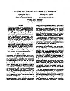
Fig. 1. Robotic table tennis setup with the ball-launcher throwing balls to the robot. In order to hit the ball to a desired position on the opponent’s court, reference trajectories are computed that facilitate the right striking motion. Such trajectories can be optimized well on the kinematics level [2], however it is hard to execute them well with inaccurate dynamics models. Iterative Learning Control using these inaccurate models leads to an efficient approach for learning to track these trajectories.
600
0
400
−2 −4 −6
0
50
100
150
40 Error norm
2
u1
x1
2
200 0 −200 −400
0
50
t
100 t
150
α α α α
= = = =
900 930 960 990
20
0
0
10
20 30 Iterations
40
Fig. 2. Learning performance of ILC, using inaccurate models without incorporating a notion of uncertainty, may not be monotonic in practice. One can observe ripples that move through the trajectory which can cause instability or damage the robot. In simulations we can create this effect easily by increasing the spectral norm of the difference between the nominal and the actual (lifted) dynamics matrices. The desired trajectory for the first state x1 is shown in dashed red on the left hand side for a two dimensional linear time invariant system. The second plot shows the ILC feedforward commands for this particular trajectory and state. The third plot shows the nonmonotonicity of the learning performance, as the mismatch scale α controlling the spectral norm of the difference is increased. Increasing α further can prevent even asymptotic stability. The solid lines were generated by direct inversion of the (lifted) model. Our proposed Bayesian approach, on the other hand, minimizing the expected cost throughout the iterations, uses the posterior over the dynamics model parameters to make more cautious decisions.
from more conservative min-max approaches, such as the robustly convergent ILC proposed in the literature (using H∞ and µ-synthesis techniques [8]). Secondly, we discuss model adaptation with linear time varying models and show that Broyden’s method [9] can be derived from Linear Bayesian Regression (LBR) as the forgetting factor goes to zero. Following the robust learning performance empirically observed in [10], we moreover discuss extensions of ILC to achieve robustness to varying initial conditions and to noise. These considerations can be quite important in practice. Rejection of such nonrepeating disturbances are shown to increase with effective weighting of the errors throughout the iterations. The final proposed approach is validated on our robot table tennis setup where we conduct experiments with dynamic hitting movements on two Barrett WAMs. Related work in the theory and practice of ILC, as well as some more general applications of learning in robotics tasks, are briefly mentioned in the next subsection. The learning control problem is stated afterwards in Section II. Model adaptation using LBR is described with various alternatives in Section III. We formulate a new cautious learning control update law, that is based on expected-cost minimization in Section IV. The resulting adaptive and cautious ILC approach, called bayesILC is described in algorithmic form in Section V, and extensions are discussed for additional robustness to nonrepetitive disturbances. In Section VI we evaluate bayesILC first in extensive simulations, showing that the proposed method is stable, efficient and can outperform other state-ofthe-art learning approaches. We then present online learning results on our robot table tennis platform. We discuss the real robot learning results in Section VII and conclude with brief mentions of promising future research directions. Derivations for the recursive and cautious learning control update introduced in Section IV are given in Appendix A. Appendix B briefly introduces the parameterization of the hitting movements for table tennis. A. Related Work Arimoto et al. [11] was one of the first to define Iterative Learning Control with the D-type update law. See [3] and [4]
for reviews. Theoretically, most ILC algorithms can be studied as a linear repetitive process using 2D-systems analysis [12]. Monotonic convergence and stability guarantees are of central importance for the practical usefulness of ILC algorithms. They are shown for example in [3], [13], [14] and recently in [8]. In practice, some of the assumptions made in the ILC literature may often be violated. Robustness to varying initial conditions are considered e.g., in [15], [16], [17]. ILC should be used along with a robust feedback controller to reject nonrepeating disturbances, see e.g., [18], [14]. Methods that learn to track (periodic or episodic) trajectories need to compensate for modeling uncertainties and other repetitive disturbances acting on the system to be controlled. However, methods that can efficiently learn the dynamics are model-based (e.g. most of optimization-based ILC [5], [3]) and at least require knowing the correct signs for the linearized dynamics of the system [19], [20]. When executing model-based learning algorithms on dynamical systems, it is essential for stability and safety to incorporate a notion of model uncertainty. Otherwise the learning algorithms can be overconfident and quickly go unstable [14]. One way to achieve a more stable performance in ILC is to filter the high-frequency updates. These robust methods are mostly known as Q-filtering [3] and typically incur a trade-off between stability and performance: the system will often fail to converge to the minimal steady-state error. In this paper, we use a different approach to increase the stability margins of model-based ILC that does not incur such a trade-off. One of the first papers introducing an optimization based ILC approach incorporating a model of the dynamics is [5]. The recursive implementation first introduced in this paper closely relates to stable plant-inversion approaches [21]. As a more recent example of model-based ILC, Schoellig et al. [22] applied a Kalman-filter based convex optimization rule that avoids direct inversion and showed its performance in quadrocopter flight. An EM-based update law was given in [23] where an impressive application of ILC to a robotic surgical task was presented. ILC has also been combined with robust observers for controlling a heavy-duty hydraulic arm during robotic excavation tasks [24].
3
Model adaptation in ILC can be studied in the context of solving nonlinear equations. Tracking a fixed reference perfectly corresponds to solving for the control inputs that drive the deviations to zero. Hence, Broyden’s method [9] and generalized secant method [25] were proposed as adaptation methods in the ILC literature to update the plant dynamics. Broyden’s method, without having access to the gradients of a black-box function f (x) = 0, maintains a Jacobian matrix approximation F. The matrix F is updated at each iteration k in order to satisfy the secant equation f k − f k−1 = Fk (xk − xk−1 ),
which can then be inverted to yield1
xk+1 = xk − F†k f k .
Convergence under restrictive assumptions have been shown for the Broyden’s method. For solving systems nonlinear equations, arguably efficiency rather than stability or monotonic convergence is of importance, and a simple trust-region approach (based on a merit function) suffices to improve stability. We will show how the Broyden’s method can be seen as a limiting case of Linear Bayesian Regression in Section III. Besides ILC, another learning framework that learns inaccurate models for control is model-based Reinforcement Learning. Including variance fully in the decision-making process can result in efficient and stable learning [26]. However such involved procedures exhibit computational runtime difficulties and have not been implemented in high-dimensional real-time robotics tasks. II. P ROBLEM S TATEMENT AND BACKGROUND Most tasks in robotics can be learned more efficiently whenever feasible trajectories are available. Learning based control approaches focus on tracking these trajectories without relying on accurate models. The goal in trajectory tracking is to track a given reference r(t), 0 ≤ t ≤ T , by applying the control inputs u(t). In dynamic robotic tasks, the references are often in the combined state space of joint positions and velocities (qT , q˙ T )T ∈ Q ⊂ R2n , and the control inputs u ∈ U ⊂ Rm are applied for each joint of the robot, i.e., m = n. The reference trajectories in table tennis, for instance, enable the execution of hitting and striking motions, i.e., forehand and backhand strikes. Such trajectories can be generated online with nonlinear constrained optimization [2]. Finding the right control inputs to track them accurately is the focus of Iterative Learning Control (ILC). 1) Linearizing an Inaccurate Model: Consider the nonlinear robot dynamics of the form ¨ = f (q, q, ˙ u), q ¨ = M−1 (q){u − C(q, q) ˙ q˙ − G(q)} + �(q, q), ˙ q
(1)
where on the right hand side are the terms due to the ˙ are the (unmodeled) rigid body dynamics model and �(q, q) disturbances that act on the robot, due to parameter mismatch, viscous friction, stiction, etc. This system can be linearized 1 Broyden’s
method can also directly update the inverse.
around a given joint space trajectory r(t), 0 ≤ t ≤ T with nominal inputs uIDM (t) calculated using the inverse dynamics model [27]. We then obtain the following linear time varying (LTV) representation ˙ e(t) = A(t)e(t) + B(t)δu(t) + d(t, u),
(2)
where the state vector is the joint angles and velocities x = [q| , q˙ | ]T , the state error is denoted as e(t) = x(t) − r(t), the deviations from the nominal inputs are δu(t) = u(t) − uIDM (t) and the continuous time varying matrices are ∂f ∂f , B(t) = . (3) A(t) = ∂x (r(t),uIDM (t)) ∂u (r(t),uIDM (t))
In the error dynamics (2) the additional term d(t, u) accounts for the disturbances and the effects of the linearization (i.e., higher order terms). We can discretize (2-3) with step size δ, N = T /δ and step index j = 1, . . . , N to get the following discrete linear system ej+1 = Aj ej + Bj δuj + dj+1 ,
(4)
where the matrices Aj , Bj are the discretizations of (3). Conventional (discrete) ILC algorithms learn to compensate for the errors incurred along the trajectory by updating the control inputs δuj iteratively. Whenever we refer to the outcome for a particular k’th iteration, we will use the first subindex for iterations and the second subindex will be used to denote the (discrete) time step, i.e., the vectors ek,j ∈ Rn , δuk,j ∈ Rm denote the deviations and control input compensations at the j’th time step during iteration k, respectively. The control commands applied at iteration k + 1 as uk+1,j = uk,j + δuk,j , are computed using the deviations ek,j at iteration k. 2) Recursive Norm-Optimal ILC: Norm-optimal ILC uses the models in (4) to minimize the next iteration errors, where the computed control inputs are optimal with respect to some vector norm. These optimal approaches can learn efficiently by taking advantage of the inaccurate models. Batch methods that compute the compensations using all the deviations, stack the model matrices together to compute (a possibly weighted and dampened) pseudoinverse of this block lower-diagonal matrix. As an alternative, some methods use convex programming to compute these optimal compensations under additional constraints. The condition of this lifted model matrix typically grows exponentially with the horizon size N and computing the pseudoinverse stably becomes very difficult. Typically downsampling trajectories restores the condition number and a stable inversion becomes much more manageable. As a better alternative, optimization based approaches, depending on the particular optimizer, may avoid computing the pseudoinverse. However such approaches can still be computationally intensive, and may not be suitable for online learning. As an alternative, the authors in [5] have shown that the direct, batch inversion of the lifted model matrix can be avoided by recursively computing the ILC compensations (in
4
min δu
N X
T eT k+1,j Qj ek+1,j + δuk,j Rj δuk,j ,
j=1
(5)
s.t. ek+1,j+1 = Aj ek+1,j + Bj uk+1,j + dj+1 .
10
5
Reduction of the ILC problem to the known LQR solution has not attracted much attention however from the control and learning communities, since it was not clear how to study stability and convergence in this formulation. III. M ODEL A DAPTATION Whenever there is model-mismatch, the linearized model cannot be assumed to hold accurately around the reference trajectory. There is hence a risk that the learning process described in the previous subsections will not be stable. As a remedy, in this section we propose a natural Bayesian adaptation of model matrices and discuss different alternatives in the context of robotics. We show first how discrete model parameter means and variances can be updated with Linear Bayesian Regression (LBR). A. Recursive Estimation of Model Matrices The observed deviations from the trajectory ek,j at iteration k can be used to update the linear models Ak,j , Bk,j , that describe the nonlinear dynamics accurately around the trajectory, to first order. Instead of estimating all the parameters together in a costly estimation procedure, the model matrices Ak,j , Bk,j can rather be updated separately for each ˆk,j j = 1, . . . , N , given the smoothened errors e ˆk,j+1 = Ak,j e ˆk,j + Bk,j uk,j + dj+1 , e
(6)
which can be rewritten using the Kronecker product and the vectorization operator as follows ˆk,j+1 − e ˆk−1,j+1 ≈ Xk,j vec [Ak,j , Bk,j ], e T
ˆk−1,j , δuk,j ] ⊗ I. Xk,j = vec [ˆ ek,j − e
If we incorporate the belief (including the uncertainty) about the linear dynamics models as Gaussian priors in LBR θ k,j = vec [Ak,j , Bk,j ], ˆk,j+1 − e ˆk−1,j+1 , yk,j = e
ρ(θ k,j |yk,j ) ∝ ρ(yk,j |θ k,j )ρ(θ k,j ),
(7)
ρ(θ k,j ) = N (θ k,j |µk,j , Σk,j ),
with a Gaussian likelihood function
0
10
20 30 Iterations
40
ρ(yk,j |θ k,j ) = N (yk,j |Xk,j θ k,j , σ I),
1) Relation to Broyden’s method: Broyden’s method [9] can be seen as a limiting case of LBR. The mean estimates in (8) are also the solutions of the following linear ridge regression problem min σ12 kyk,j − Xk,j θk22 + (θ − θ k,j )Σ−1 k,j (θ − θ k,j ), θ
and as σ 2 → 0 we get the (weighted) Broyden’s update for one iteration, which, written in vectorized form, is solving independently for every time step min (θ − θ k,j )Σ−1 k,j (θ − θ k,j ), θ
s.t. yk,j = Xk,j θ.
(9)
Broyden’s method is too sensitive to the sensor noise in robotics tasks as it satisfies the secant rule (9) exactly. On the other hand, LBR in (8) for fixed noise parameter σ 2 , is using all of the past iteration data equally. The norm of the covariance decreases monotonically in each update. For unknown dynamical systems that are highly nonlinear but smooth, to prevent premature shrinking of the covariance matrix, a better alternative is to set an exponential weighting in the adaptation. For a fixed forgetting factor λ ∈ [0, 1], the update in (8) becomes
µk,j = λΣk,j Σ−1 k−1,j µk−1,j +
the models parameter means µk,j and variances Σk,j can be updated as (8)
Smoothened position and velocity error estimates can be obtained, for example, using a zero-phase Butterworth filter.
50
Fig. 3. Broyden’s method [9], which can be considered as an adaptation framework within ILC, is a limiting case of Linear Bayesian Regression (LBR). As the forgetting factor λ of an exponentially weighted LBR model goes to zero, LBR transitions to the Broyden’s method. Broyden’s method is very sensitive to noise and adapts very aggressively. Throughout the paper, we discuss and evaluate several adaptation laws, that are less sensitive to noise but are still flexible. The Figure shows the evolution of the identification error norm for an unknown linear time varying system. The Frobenius norm of the difference between the adapted model matrices (Ak,j and Bk,j ) and the actual (fixed) matrices are plotted for each iteration k = 1, . . . , 50.
−1 −1 , Σk,j = ( σ12 XT k,j Xk,j + λΣk−1,j )
2
−1 −1 , Σk,j = ( σ12 XT k,j Xk,j + Σk−1,j ) � � T 1 µk,j = Σk,j Σ−1 k−1,j µk−1,j + σ 2 Xk,j yk,j .
lbr broyden λ = 0.8 λ = 0.4 λ = 0.01
15 Error norm
one pass) using the Linear Quadratic Regulator (LQR) for disturbance rejection [28]. After estimating the disturbances dj+1 at the k 0 th trial, the optimal control problem for tracking a desired trajectory can be written as
T 1 σ 2 Σk,j Xk,j yk,j .
(10)
The forgetting factor λ is used to perform exponential weighting of the previous iteration data. As λ → 0, we get the (unweighted) Broyden’s method2 , and as λ → 1, (10) reduces to (8). See Figure 3 for an illustration. 2 Unlike the case where σ 2 → 0, this equivalence is valid for all the subsequent iterations as well. It can be seen more easily from the filter form of (10).
5
B. Imposing structure The structure in the forward dynamics model is not considered in the update rule (10): change in the control inputs directly affects the instantaneous joint accelerations, and only indirectly the joint velocities in the future time steps. By differentiating the smoothened joint velocities, one can instead impose the following model ¨ k,j − q ¨ k−1,j = Ak (δj)ek,j + Bk (δj)δuk,j , q where we dropped the hat for notational simplicity. The continuous model matrices Ak (δj), Bk (δj) are members of a reduced parameter space, i.e., Ak (δj) ∈ Rn×2n , Bk (δj) ∈ Rn×m , j = 1, . . . , N . After estimating the continuous model parameter means and variances as in (8), they can be discretized (as discussed before) to form the discrete model parameter means Ak,j ∈ R2n×2n , Bk,j ∈ R2n×m and covariances Σk,j . As an alternative, note that the rigid body dynamics (1) is parameterized by the link masses, three link center of mass values and six inertia parameters. A total of ten parameters are used for each link to fully parameterize the inverse dynamics model which can be stacked for each j = 1, . . . , N to form the regression model ˙ k, Q ¨ k )θ k , Uk ≈ Y(Qk , Q
(11)
where θ k ∈ R10n appears linearly. Based on the iteration performance (joint position, velocity and acceleration estimates) only the link parameters are updated with LBR as in (8). The forward dynamics model3 (1) can then be used to sample the means and variances of the continuous LTV matrices, e.g., using Monte Carlo sampling. Discretization as discussed above converts the continuous model parameter means and variances into their discrete form. An advantage of this approach is to compress learning to a lower dimensional space, reducing the variance of the updates at the cost of an introduced bias. Moreover, since the link parameters are invariant throughout the iterations, such an update avoids the flexible yet independent adaptation of the model matrices for each j, and the necessity of introducing a forgetting factor. IV. C AUTIOUS L EARNING C ONTROL The posterior model covariances Σk,j can be used to make more cautious decisions within a stochastic control framework. The uncertainty of the model parameters can be seen as a multiplicative noise model and the ILC optimality criterion (5) can be extended to include expectations over them. The multiplicative noise model, unlike the additive noise case, does not lead to certainty-equivalence: the covariance estimates are 3 The
ˆT ˆk,j ) ≤ P(eT k+1,j Qj ek+1,j ≥ e k,j Qj e
E[eT k+1,j Qj ek+1,j ] ˆT ˆk,j e k,j Qj e
,
which follows from Markov’s inequality. Minimizing the upper bound forces the probability of nonmonotonicity to be low as well. 1) Cautious ILC: For the expected cost case, where the expectation is taken over the random variables Ak,j and Bk,j , for each j, the optimality criterion min δu
N X
T EAk,j ,Bk,j [eT k+1,j Qj ek+1,j +δuk,j Rj δuk,j ],
j=1
s.t. ek+1,j+1 = Ak,j ek+1,j + Bk,j uk+1,j + dj+1 , can be solved recursively using dynamic programming [29] δuk,j = Kk,j ek+1,j − Φ−1 k,j `k,j , Kk,j = −Φ−1 k,j Ψk,j ,
Φk,j = EBk,j [BT k,j Pk,j+1 Bk,j ] + Rj ,
Ψk,j = EAk,j ,Bk,j [BT k,j Pk,j+1 Ak,j ],
˙ θ)q˙ + G(q; θ), u = M(q; θ)¨ q + C(q, q;
�T T T Uk = uT , k,1 , uk,2 , . . . , uk,N �T � (l) (l)T (l)T (l)T , l = 0, 1, 2, Qk = qk,1 , qk,2 , . . . , qk,N
incorporated in the decision rule. To see how the expected cost minimization leads to caution, note that
forward dynamics model (1), unlike the inverse dynamics (11), depends nonlinearly on the link parameters.
T `k,j = EBk,j [BT k,j Pk,j+1 (Bk,j uk,j +dj+1 )+Bk,j bk,j+1 ], (12) where bk,j and the Ricatti matrices Pk,j evolve backwards according to −1 Pk,j = Qj + Mk,j − ΨT k,j Φk,j Ψk,j ,
Mk,j = EAk,j [AT k,j Pk,j+1 Ak,j ], ¯ T (bk,j+1 +Pk,j+1 (Bk,j uk,j +dj+1 ))], bk,j = EA ,B [A k,j
k,j
k,j
starting from Pk,N = QN and bk,N = 0. The random closed loop system dynamics is given by the matrices ¯ k,j = Ak,j + Bk,j Kk,j . A By a direct comparison to the LQR solution to (5), it can be seen that the control input compensations δuk,j in (12) are computed similarly, with the appropriate expectations added. The ILC update is decomposed into two: a currentiteration feedback term ufb = Kk,j ek+1,j calculated using the iteration dependent Riccati equations and a feedforward, purely predictive term uff = −Φ−1 k,j `k,j , solved backwards for each j = 1, . . . , N . The feedforward terms are responsible for compensating for the estimated random disturbances dj , calculated using (6). Cautious update (12) can be implemented without explicitly calculating the disturbances. If the disturbances are taken as ˆk,j of the last random variables defined via the filtered errors e iteration ˆk,j+1 − Ak,j e ˆk,j − Bk,j uk,j , dj+1 = e the recursion can be simplified by introducing ν k,j = bk,j + Pk,j ek,j .
6
The feedforward and feedback compensations δuk,j can then directly be computed as δuk,j = Kk,j (ek+1,j – ek,j ) – Φk,j EBk,j [BT k,j ν k,j+1 ], (13) T ¯ ν k,j+1 ] + Qj ek,j . ν k,j = EA ,B [A k,j
k,j
k,j
See Appendix A for a detailed derivation. Equation (13) easier to implement, since the disturbances do not need to be estimated explicitly. The compensations δuk,j are added to the total control inputs applied at iteration k. In an adaptive implementation, the feedback components of the update, Kk,j (ek+1,j −ek,j ), does not completely subtract the previous feedback controls Kk−1,j ek,j from the total control inputs, as the feedback matrices are also adapted over the iterations. Typically ILC is used to feed the past errors along the trajectory (filtered and multiplied with a learning matrix) back to the system for the next trial as feedforward compensations. A well designed feedback controller, whenever available, is only used to reject nonrepeating disturbances and to stabilize the system in the time domain. The recursive implementation (13), on the other hand, readily provides and updates a feedback controller based on past performance. From here on, we will refer to the feedforward part of (13) as δuk,j , keeping the feedback control separate. 2) Computing the Expectations: The expectations appearing in (12) can be calculated given the covariances Σk,j of the parameters, ˜ k,j + Rj , Φk,j = Φ n n X � � X c,a d,b c,a d,b ˜ a,b = Pc,d E[B ]E[B ]+σ(B , B ) , Φ k,j k,j+1 k,j k,j k,j k,j c=1 d=1
Ψa,b k,j =
n n X X c=1 d=1
Ma,b k,j
=
n X n X c=1 d=1
� � c,a d,b c,a d,b Pc,d k,j+1 E[Bk,j ]E[Ak,j ] + σ(Bk,j , Ak,j ) ,
� � c,a d,b c,a d,b Pc,d k,j+1 E[Ak,j ]E[Ak,j ] + σ(Ak,j , Ak,j ) ,
where the upper indices a, b denote the corresponding entry of the matrix appearing on the left hand side. The covariance matrices Σk,j contain the scalar covariance terms σ(·) on the relevant entries, i.e., (a−1)n+c,(b−1)n+d
d,b σ(Ac,a k,j , Ak,j ) = (Σk,j ) d,b σ(Bc,a k,j , Ak,j )
,
n2 +(a−1)n+c,(b−1)n+d
= (Σk,j )
2
2
,
n +(a−1)n+c,n +(b−1)n+d
d,b σ(Bc,a k,j , Bk,j ) = (Σk,j )
.
The indexes of Bk,j covariances start from n since the model matrix parameters in (7) are vectorized starting from Ak,j . 2
V. O NLINE I MPLEMENTATION In this section we algorithmically describe the recursive, adaptive and cautious bayesILC proposed in the last two sections in detail, with the extensions for an online robot learning application. We will consider tracking table tennis trajectories as our application of choice. The online learning algorithm is readily applicable to similar dynamic tasks with real-time constraints, such as throwing, catching skills in sports or fast, demanding manufacturing tasks.
Algorithm 1 Recursive, adaptive and cautious bayesILC. Require: f nom , rj , λ, � > 0, Qj � 0, Rj � 0, Σ0,j � 0 ˙ 0 = 0. 1: Move to initial posture q0 = r0 , q 2: Initialize k = 1, δu0,j = 0, j = 1, . . . , N 3: Compute mean dyn. parameters µ0,j by linearizing f nom 4: Compute feedback K0,j = LQR(Qj , Rj , µ0,j , Σ0,j ) 5: Execute with inv. dyn. uIDM and feedback K0,j ˆ0,j ) 6: Filter errors with a zero-phase filter (output: e 7: repeat \\ ILC operation PN T ˆk,j Qj e ˆk,j 8: Compute cost Jk = j=1 e 9: Compute δuk,j , Kk,j recursively using (12) – (13) 10: Update feedforward controls uk+1,j = uk,j + δuk,j 11: Execute with uIDM,j + uk+1,j and feedback Kk,j 12: Observe errors ek,j = xk,j − rj ˆk,j ) 13: Filter errors with a zero-phase filter (output: e 14: Update model µk,j , Σk,j using (10) 15: k ←k+1 16: until Jk < � The proposed ILC framework is summarized in Algorithm 1. Before entering the ILC loop (lines 7 − 16), the trajectory is executed with inverse dynamics and time-varying LQR feedback (line 5). The errors along the trajectory are filtered with a zero-phase filter (line 6). The adaptive and cautious bayesILC then updates the feedback control law as well as the feedforward control inputs recursively (line 9). From the first iteration onwards, the means and the covariances of the model matrices are updated (line 14) before computing the feedforward input compensations δuk,j and the feedback matrices Kk,j . Based on the forgetting factor λ, the model adaptation strikes a balance between the prior model parameter ˆk,j+1 − e ˆk−1,j+1 observed distribution and the data yk,j = e in iteration k. We discuss the effects of the forgetting factor and the different model adaptation strategies in more detail in Section VI. The practitioner, wary of the model inaccuracies, can increase robustness and ensure stability by setting large diagonal terms for the initial covariance of model uncertainty, Σ0,j = γI, γ � 1, j = 1, . . . , N . Moreover, setting large covariances initially helps to observe the inaccuracies of the model and the noise statistics. The covariance will be suitably decreased over the iterations, as adaptation (10) updates the linear models. Observing the noise statistics over the iterations can further help in the design of a good zero-phase filter to reject noise. The proposed update law takes advantage of the learning efficiency and computational advantages of model-based recursive ILC while being cautious with respect to model mismatch. The computational complexity of the recursive update is O(N n3 ) as opposed to batch norm-optimal ILC, where the batch pseudoinverse operation typically incurs O(N 3 n3 ) complexity. The batch model-based implementation using the lifted-vector form [3] inverts the input-to-output matrix F, Uk+1 = Uk − F† Ek ,
T T Ek = eT k,1 , ek,2 , . . . , ek,N
�T
,
(14)
7
Algorithm 2 ILC improving execution of robot table tennis hitting movements online. Require: q0 , f ball , bayesILC(. . .) (see Algorithm1) ˙ 0 = 0. 1: Move to initial posture q0 , q 2: Predict ball trajectory bj using f ball 3: Compute trajectory rj given q0 and bj , j = 1, . . . , N 4: Setup bayesILC (lines 2 − 4) 5: repeat \\ fixed ballgun throws balls at a constant rate 6: Execute strike with uILC and LQR feedback K 7: Return to q0 with high-gain PD control and linear traj. 8: Update uILC and K with bayesILC (lines 9 − 14) 9: until ballgun is moved
where the submatrices of the input-to-output matrix F are Ai−1 . . . Aj Bj−1 , j < i, Bj−1 , j = i, F(i,j) = (15) 0, j > i. The condition of the lifted model matrix (15) grows exponentially with N and inverting it quickly becomes numerically unstable.
1) Implementation for Tracking Table Tennis Trajectories: The online learning framework for robot table tennis is described in Algorithm 2. Whenever a ball is initialized from a fixed ballgun with constant settings, located at b0 , the trajectory generation framework will compute a particular striking trajectory (lines 2 − 3) to intercept and hit the ball in real time. See Appendix B for an overview of the trajectory generation pipeline. ILC can then be initialized (line 4) by linearizing the dynamics model f nom around the computed trajectory points rj , j = 1, . . . , N . ILC needs to be initialized only once, as long as the computed trajectory is capable of returning the ball to the opponent’s court. The approximately 8cm radius of the racket can cover for the inconstancy of the ballgun up to a certain degree. Whenever the striking trajectory is executed (line 6), a returning trajectory will bring the arm back (line 7) from the current state to the fixed initial posture, q0 . The returning trajectory can be as simple as a linear trajectory in the joint space. The consistency provided by the fixed ballgun in our setup, shown in Figure 1, allows us to use ILC to track invariant trajectories over the iterations. For a good performance in table tennis, the striking parts of these hitting movements need to be tracked accurately. The strikes are initially tracked with computed-torque inverse dynamics feedforward control commands and the additional LQR feedback. The feedback law is computed for this purpose by linearizing the nominal dynamics model around the striking part of the reference trajectory. After a strike is completed, feedback will switch to PD-gains for the returning trajectory and the arm will come back close to q0 . Learning with ILC can then take place (line 8) while waiting for another incoming table tennis ball. The striking trajectory in table tennis is only an intermediary and does not need to be precisely tracked for a successful performance. In general, for hitting and catching tasks, the
task performance depends critically on reaching the desired joint positions and velocities at the final time. A good performance along the trajectories is a means to this desired end: if feedback keeps the system stable around the trajectories, and the (linearized) models are reasonably valid around the trajectories, convergence to desirable performance levels can be rapid. 2) Coping with Varying Initial Conditions: Execution errors in tracking the reference trajectory (including the returning segment) prevents the robot from initializing in each iteration at the same state. Putting very high feedback gains on the returning trajectory or waiting long enough may suffice to initialize the system close to desired initial conditions, but in some occasions, none of these options may be desirable or available. For example, a robot practicing table tennis with a fixed ballgun running at a fixed rate, may not have time to initialize its desired posture accurately. Starting from varying initial conditions xk,0 = [q|k,0 , q˙ |k,0 ]T one can consider updating the hitting movement rj to take the robot to the same hitting state. For such online updating of trajectories, the invariant trajectory parameters p can be used to generate the trajectory from the current joint values. The reference control inputs uIDM can then be recomputed based on the nominal inverse dynamics model. With this correction the total feedforward control commands uILC at iteration k+1 are re-computed as uILC,j = uk+1,j + uIDM,j (˜rj ) − uIDM,j (rj ),
(16)
where ˜rj is the updated trajectory starting from the perturbed initial state x0 + δxk,0 . Using this simple adjustment (16), the stability of the learning performance can be greatly improved. VI. E VALUATIONS AND E XPERIMENTS In this section, we demonstrate the effectiveness of the ILC algorithm bayesILC presented in Algorithm 1 and described in detail in Section V in the context of tracking table tennis trajectories. We validate the proposed learning control law first in extensive simulations with linear and nonlinear models. In the last section we show real robot experiments with two seven degree of freedom Barrett WAM arms for tracking table tennis striking movements. A. Verification on Toy Problems Stability is an important issue in the implementation of different learning controllers in real robot tasks. As a result, we setup extensive simulation experiments to validate the stability and robustness of our learning approach. We also discuss in detail the advantages of the recursive formulation over the batch pseudo-inverse ILC (14). 1) Random Linear Models: We generate here random linear models and random trajectories drawn from Gaussian Processes (GP) with squared exponential kernels. More specifically, the elements of the linear time varying (LTV) model matrices Aj , Bj are drawn from (n+m)n uncorrelated GPs. The hyperparameters (scale, noise and smoothness parameters) of these GPs are drawn independently from normal distributions
8
Error norm
20 15
recursive ILC batch ILC
10
bayesILC nonadaptive cautious ILC
10 5
5 0
5 10 Iterations
0
2
4
6 8 Iterations
10
Fig. 4. ILC in recursive form is evaluated on random linear time varying (LTV) systems. Results are averaged over ten experiments, where for each experiment, trajectories, nominal models and actual models are drawn randomly from Gaussian Processes. The performance of the batch pseudo-inverse ILC (14) is shown in the red line. Numerical stability issues prevent it from stabilizing at steady state error, whereas recursive ILC (blue line) converges stably. If the model mismatch is increased, at some point, recursive ILC also diverges. Applying caution without adaptation is not enough to converge to steady state error. Cautious and adaptive bayesILC, on the other hand, applying the updates (8) and (13) iteratively, is very effective and shows a stably convergent behaviour.
with fixed means and variances. Moreover, random perturbations of these models (drawn the same way from (n + m)n uncorrelated GP’s) are generated to construct nominal models. Using the proposed random disturbance generation scheme, we can average the results and construct error bars for different ILC algorithms. The performance of the recursive implementation (i.e., Equation (13) with zero covariances and no adaptation) is shown in Figure 4 on the left hand side, where the results are averaged over ten different trajectories and models. The dimensions of the models are n = 2, m = 2, and the horizon size is set to N = 120. For the LQR and ILC calculations, R = 10−6 I and the weighting matrix Q was set to the identity. In this case, the batch model-based implementation using the pseudo-inverse (14) is not stable at all without feedback. Applying LQR feedback and adding current iteration ILC in Figure 4 improves the performance (red line in Figure 4), but numerical issues (i.e., large condition number) in inverting the large model matrix F in lifted form (15) prevents it from stabilizing at steady state error. Tracking performance throughout the experiments is measured with respect to the 2-norm of the deviations Ek . For the simulation results in Figure 4, the spectral norm of the difference between the nominal and the actual models are each set to ασmin (F) where α = 100. Increasing α further increases the probability that the model-based ILC is not monotonically convergent for some trial. For example, one can observe asympotically but not monotonically convergent ILC behaviour when setting α = 990 for a particular model and trajectory shown in Figure 2. Increasing α futher can prevent even asymptotic stability. Especially in these cases of high model mismatch, the proposed adaptive and cautious bayesILC offers a stable and convergent ILC behaviour. In Figure 4 on the right hand side, we consider the case where α = 1000. Recursive ILC that is also cautious does not show a stable convergent behaviour, whereas recursive ILC that is not cautious (i.e., covariance of the LTV matrices are zero) is not stable at all.
Cautious and adaptive bayesILC, on the other hand, using LBR (λ = 0) to update the discrete LTV matrices Ak,j , Bk,j , shows a monotonic learning performance. The results are again averaged over ten different models and ten trajectories. For LBR, the initial covariances in (8) are set to Σ0,j = γI for all j = 1, . . . , N , where γ = 104 and the noise covariance is σ 2 = 1. Changing the exponent of the initial covariance, or reducing the forgetting factor λ in this case, can lead to a reduced or unstable learning performance. 2) Gaussian Process Dynamics: The performance of the proposed algorithm bayesILC is evaluated next over random nonlinear models. In these set of experiments, we sample the states from n uncorrelated GPs with squared exponential kernels and random linear mean functions. The hyperparameters of these GPs are randomized as before. By sampling from such random nonlinear models, we can test the proposed algorithm under nonlinear uncertainties and noisy outputs. The actual model is simulated as follows: 1) Random reference inputs vj ∈ Rm , j = 1, . . . , N are drawn K times from m GPs. 2) n oracle GPs are used to sample f (xj , vj ) and the generated dynamics is integrated (starting from zero initial conditions) using forward Euler, dt = 1/N , to form K trajectories. The GPs are conditioned during this process on the generated states xj and inputs vj . These n oracle GPs constitute the actual but unknown nonlinear dynamics model. Nominal models can be easily generated by using the predictions of the oracle GPs at a subset of the state space. The construction of a nominal model is described in detail below: 1) Another set of control inputs uj , j = 1, . . . , N are drawn from GPs. 2) The mean predictions f (xj , uj ) of the oracle GPs at uj are used to evolve these control inputs (as in step 2 of the actual model). 3) The n separate model GPs (with same hyperparameters as the oracle) are conditioned on the resulting trajectory, i.e., the input pairs (xj , uj ) and the outputs f j = (xj+1 − xj )/N for each time step j = 1, . . . , N . 4) The mean derivative of the model GPs are calculated analytically (using the kernel derivatives). Discretized time varying matrices Aj , Bj and their variances Σ0,j are constructed for each j = 1, . . . , N , based on the mean and variance of the GP derivatives. By sampling K = 20 trajectories for the conditioning of oracle GPs, we can cover a significant part of the state space in n = 2 dimensions. For each ILC iteration thereafter, the mean predictions are used as in step (2) to evolve the trajectory, but without further conditioning of the model GPs. Instead, adaptation is performed as before with LBR, replacing the steps (3 − 4). We can thus avoid the expensive online GP training. Figure 5 shows the learning performance for a horizon size of N = 20. The dimensions of the system is same as before, n = 2, m = 2 and R = 10−6 I, Q = I. The results are averaged again over ten experiments. In this nonlinear setting, the recursive ILC that is not cautious shows an unstable behaviour (not shown in Figure 5). Adding adaptation without caution (i.e.,
9
bayesILC nonadaptive cautious ILC
Error norm
Error norm
10
5
z
−0.5
1
−1
0 0
Discrete LTV Continuous LTV Link parameters
2
0
5
10 Iterations
15
20
Fig. 5. The proposed ILC algorithm is evaluated on random nonlinear systems. Results are averaged over ten experiments, where for each experiment, trajectories and dynamics along these trajectories are drawn from Gaussian Processes. Recursive ILC that is not cautious shows an unstable behaviour (not shown in the Figure). Adding adaptation without caution is also not stable. Cautious and adaptive bayesILC, on the other hand (blue line), shows a stable convergent learning performance, whereas purely cautious ILC (brown line) is divergent for some of the trajectories.
using the covariances of the LTV matrices) is not stable for some trajectories and can diverge (brown line). Cautious and adaptive bayesILC, on the other hand, using LBR to update the discrete LTV matrices, shows again a stable convergent learning performance, whereas purely cautious ILC is seen to be worse. For LBR, the initial covariances in (8) are again set to γ = 104 times the identity and the noise covariance is σ 2 = 1. The best performance is reached when the forgetting factor is set to λ = 0.9. As before, changing the exponent of the initial covariance, or the forgetting factor, can lead to a reduced or unstable learning performance. 3) Barrett WAM Model: We next test ILC on striking movements (29) for a seven degree of freedom Barrett WAM simulation model. In the simulations, the robot is started from a fixed initial state q0 . The initial posture is chosen from one of the center, right hand side or left hand side resting postures of the robot. The striking parameters (30) are then optimized, based on an incoming table tennis ball with a randomly chosen incoming position and velocity. The link parameters of the Barrett WAM forward dynamics model used to simulate actual trajectories are perturbed randomly to construct nominal models for ILC. The linearization procedure described in Section II produces LTV nominal models that can be used by ILC to reduce the deviations from the desired (fixed) striking movement over the iterations. The randomization during the optimization guarantees that a variety of hitting movements are tracked throughout the experiments. The performance of the proposed ILC approach bayesILC with three different adaptation laws is then evaluated over the striking segment of the optimized (striking and returning) trajectories. The convergence results are averaged over ten such striking movements, as shown in Figure 6. The adaptation of discrete and continuous LTV models are shown in blue and red, respectively, while the adaptation of link parameters is shown in black. Forgetting factor was set to λ = 0.8 for all of the adaptation laws. Initial covariances are set to Σ0,j = 104 I for continuous and discrete LTV
5 Iterations
10
0.5 0.5
0
0
Fig. 6. The performance of the adaptive and cautious ILC algorithm bayesILC on the Barrett WAM model is shown in the left hand side. The results are averaged over ten different strikes and three different initial postures. Three different adaptation laws are considered, adaptation of discrete and continuous LTV models are shown in blue and red, respectively, while the adaptation of link parameters is shown in black. Forgetting factor was set to λ = 0.8 for all of the adaptation laws. One of the desired trajectories, shown in dashed red on the right hand side, is tracked very closely in the final iteration. The blue markers correspond to the time profile of the motion, which are drawn uniformly spaced, one for each 80 milliseconds.
model adaptation laws, while for link parameters, the initial covariances are Σ0,j = 1010 I. The weights of the cautious ILC update (13) is set to R = 10−2 I, Q = I. After updating the link parameter means and variances, we use an auto-differentiation tool (ADOL-C library in C++) together with sampling to approximate the distribution of forward dynamics (1) derivatives Ak,j , Bk,j . More specifically, the forward dynamics is differentiated (with respect to joint positions, velocities and control inputs) at 100 link parameter samples drawn from the posterior distribution (i.e., normal distribution with means and variances given by (8)) online. This sampling procedure generates a reasonable approximation of posterior derivative means and variances. In table tennis, if the robot arm follows the assigned reference trajectory precisely it will hit the ball with a desired velocity at the desired time. We can see in the right hand side of Figure 6 that an initial attempt (blue curve) falls short of the reference trajectories (dashed curve). The percentage of the balls that are returned to the opponent’s court are close to zero. ILC then modifies the control inputs to compensate for the modeling errors. In the last attempt the reference trajectory is executed almost perfectly. The accuracy of the table tennis task increases to %95, on average. Figure 7 shows the adjusted control inputs for one striking movement. The recursive ILC (without adaptation or caution) is convergent for some of the hitting movements in Figure 6. However, similar to the previous simulation examples, the recursive form of the ILC update, depending on the accuracy of the model along the trajectories, can fail to converge for some trajectories (not shown in the Figure). The proposed recursive, adaptive and cautious algorithm bayesILC, with the three adaptation laws shown in Figure 6, shows a better and faster convergence, for a variety of trajectories. The ILC experiments shown in Figures 6–7 reset the initial posture always to the same desired posture q0 . Next, we consider non-repetitive disturbances around the desired initial posture. This would mean, physically, that the robot is not initialized accurately around the resting posture. Comparisons to the baseline (black line) in Figure 8 illus-
10
0.4
0.6
0.8
1
0.2
0.4
0.6
0.8
1
0.2
0.4
0.6
0.8
1
0.2
0.4
0.6
0.8
1
0.2
0.4
0.6
0.8
1
0.2
0.4
0.6
0.8
1
0.2
0.4
0.6
0.8
1
q2
0.2
0.4
0.6
0.8
1
0
0.2
0.4
0.6
0.8
1
0 0.5 0 −0.5 −1 0 3 2 1 0 0 0 −1 −2 −3 0 4 2 0 −2 0
0.2
0.4
0.6
0.8
1
0.2
0.4
0.6
0.8
1
0.2
0.4
0.6
0.8
1
0.2
0.4
0.6
0.8
1
0.2
0.4
0.6
0.8
1
0 −1 −2 −3 4 2 0 −2
q7
q˙7
q6
q˙6
q5
q˙5
q˙4
q˙3
q3 q4
B. Real Robot Table Tennis 0
q˙2
0.2
4 2 0 −2
Time (s)
Time (s)
Fig. 7. Joint trajectories for a hitting movement on the Barrett WAM model. The reference trajectories, shown in dashed red, are tracked very closely with ILC in the final iteration, shown in blue.
Final cost
3
ILC with trajectory adaptation ILC without trajectory adaptation
2 1 0
1
2
3 4 Iterations
5
Fig. 8. Simulation results illustrating the additional robustness to varying initial conditions whenever the trajectories (states and control references) are adapted according to (16) (blue line). Note the unstable performance of ILC without such adaptation (black line), which keeps the references rj and the inverse dynamics inputs uIDM,j fixed.
trate the additional robustness whenever the trajectory adaptation (16) is employed. We adapt the metric for this comparison according to the task: the costs indicated are the final costs (for hitting the incoming ball at the desired joint positions with desired joint velocities), not the full costs incurred along the reference trajectory. Note especially the faster convergence and increased accuracy of the proposed method with the reference trajectory and input adaptation (blue line). More robust performance is obtained by adapting the trajectories rj and uIDM,j , which, in addition to performing better, shows much lower variance compared to the baseline. In practice trusting the model too much at the beginning of the trajectory leads to the amplification of initial errors. Nonrepetitive starting postures violate the initial condition assumption typical of standard ILC updates. In this case, the feedback matrices Kk,j , as opposed to the feedforward input updates δuk,j , play a bigger role in the learning stability at the beginning of the trajectories, j � N .
Finally we perform experiments on our robotic table tennis platform, see Figure 1, where two seven degree of freedom (DoF) cable-driven, torque-controlled Barrett WAM arms (Ping and Pong) are hanging from the ceiling. The custom made Barrett WAM arms are capable of high speeds and accelerations (approx. up to 10m/s2 in task space). Standard size rackets (16 cm diameter) are mounted on the end-effector of the arms as can be seen in Figures 10 and 11. A vision system consisting of four cameras hanging from the ceiling around each corner of the table is used for tracking the ball [30]. A ball launcher (see Figure 1) is available to throw balls accurately to a fixed position inside the workspace of the robots. The incoming ball arrives with low-variability in desired positions and higher-variability in ball velocities. The whole area to be covered amounts to about 1 m2 circular region surrounding an initial centered posture of the robots. The realistic simulation environment SL [31] acts as both a simulator and as a real-time interface to the Barrett WAMs in our experiments. The initial positioning is given by a PD controller with high gains on the shoulder joints, which is then toggled off during the experiments with the striking movements, as summarized in Algorithm 2. The high gain PD controller used to initialize the robots was also tested for tracking the striking movements, see Figure 9. When ILC is applied on top of the PD controller, the learning quickly stagnates, leading to oscillations in some of the joints. Instead, a low-gain LQR feedback law is computed for the striking part of the movement with a linearized nominal dynamics model (4). The weighting matrices for this purpose are set to identity, Q = I, and the constant penalty matrix is chosen as R = 0.05I. Decreasing the scaling of the penalty matrix to 0.03 causes oscillations in the elbow joint, indicating that the nominal model is not very accurate. At the cost of larger initial error, we suggest increasing the input penalties R to improve the stability of ILC in other high degrees-of-freedom
−0.5 z
q˙1
q1
1 0.8 0.6 0.4 0.2 0 0 0 −1 −2 −3 0 0 −0.2 −0.4 −0.6 −0.8 −1 0 2 1.8 1.6 1.4 0 1 0 −1 −2 0 1 0 −1 −2 0 3 2 1 0 0
−1 0.2
0 x
−0.2 −0.4
−0.6
−0.8 y
Fig. 9. An example of a striking movement for table tennis is shown in red. The blue markers correspond to the time profile of the motion, which are drawn uniformly, one for each 80 milliseconds. Executing this movement well with the Barrett WAM will lead to a good hit. Control errors in tracking lead to a poor hitting performance, shown in blue. High-gain PD feedback was used to track the reference in this real robot example. The tracking errors can be decreased efficiently and stably by applying the proposed recursive, cautious and adaptive ILC update bayesILC.
11
Fig. 10. The Barrett WAM (a.k.a. Ping) is initialized in our experiments in three different starting postures. We make controlled experiments with a simulated ballgun, and generate many different hitting movements, two of them are shown in the above images. The proposed algorithm bayesILC leads to an efficient and stable learning approach for tracking these hitting movements. The right hand side starting posture can be seen on the upper left image. Initially, before learning with ILC starts, the robot performs poorly, and the hitting posture of the robot is shown in the upper central image. After five iterations, the hitting posture is corrected significantly as shown in the upper right image. Similarly, the bottom three images show the operation of the ILC for another trajectory, where the starting posture is fixed on the left hand side of the robot.
Fig. 11. The Barrett WAM (a.k.a. Pong) is initialized in our experiments in three different starting postures. We make controlled experiments with a simulated ballgun, and generate many different hitting movements, one of them is shown in the above images. The proposed algorithm bayesILC leads to an efficient and stable learning approach for tracking these hitting movements. The left hand side starting posture can be seen on the left image. Initially, before learning with ILC starts, the robot performs poorly, and the hitting posture of the robot is shown in the central image. After five iterations, the hitting posture is corrected significantly as shown in the upper right image.
robotics applications. After the visual system outputs a ball estimate, a ball model can be used along with an Extended Kalman Filter to predict a ball trajectory. The ball model accounts for some of the bouncing behavior of the ball and air drag effects. If the predicted ball trajectory coincides with the workspace of the robot, the motion planning system has to then come up with a trajectory that specifies how, where and when to intercept the incoming ball. Desired Cartesian position, velocity and orientations of the racket at the hitting time T impose constraints on the seven joint angles and seven joint velocities of the robot arm at T . Along with the desired hitting time T (or the time until impact), these fifteen parameters are used to generate third-order joint space polynomials. These movements can be optimized online in 20 − 30 milliseconds [2], or loaded from a lookup table. In the ILC experiments, the parameters in the lookup table are used without interpolation, to make sure that the same trajectory can be used for balls deviating slightly from their stored values. We make sure that the lookup table is dense enough and that the ballgun is fixed.
resting posture in Trest = 1.0 seconds. PD feedback control is turned on again for this returning part of the trajectory. When the returning trajectory is executed, SL main thread running the inverse dynamics computations will continue to keep the arms stable around the resting posture, while another thread is detached to run the ILC update4 . The ILC loop terminates successfully whenever the computed feedforward updates are within the respective torque limits. After a successful termination, if the actual posture is within 0.1 radians distance of the resting posture, the LQR feedback will be turned on again and the robots will start moving to track the same striking motion. We use a simulated ball to make more controlled experiments, focusing on the control aspect in more detail. If the striking robot movements are executed accurately, then the ball in simulation will be returned close to a desired position on the opponent’s court. At different points in time we have identified three different sets of link parameters for rigid body dynamics. We can use these parameterizations of rigid body dynamics as potential nominal models to kick-start the learning process. We tested these nominal models first in slowed down hitting
Some examples of the generated trajectories are shown in Figures 10 and 11. After a strike, a linear joint trajectory is computed that will take the robots from the current state to the
4 Code is available in the public repository https://gitlab.tuebingen.mpg.de/ okoc/learning-control along with the test scripts used to generate the plots in the previous subsections.
12
2
4
6
8
10
q2
2 1 0 −1 −2
0
2
4
6
8
10
2 1 0 −1 −2
0
2
4
6
8
10
0
2
4
6
8
10
−1 −1.5 −2 −2.5 −3
0
2
4
6
8
10
1 0.5 0 −0.5 −1
0
2
4
6
8
10
0
2
4
6
8
10
2 1.5 1 0.5 0
q7
q6
q5
q4
0
q3
q1
0.4 0.2 0 −0.2 −0.4
1 0.8 0.6 0.4 0.2 0
Time (s) Fig. 12. Robot experiment results for cautious and adaptive bayesILC, shown for a particular reference trajectory. The ten iteration results are concatenated for convenience. The desired joint trajectories correspond to a hitting movement on the Barrett WAM. The reference trajectories, shown in red, are tracked very closely with ILC in the final iteration, shown in blue. Final cost goes down to 0.20 in the last iteration.
movements, where a slow down rate of two means that the number of trajectory points double while the hitting time is held fixed. Cutting down the trajectories to an initial subset of the movement to restrict potential instabilities, or initial masking of some of the joints during ILC updates, are other techniques that we have employed to evaluate these nominal models in a careful manner. Of the three models, only one of them was suitable for the local learning that ILC provides. This model is further adapted with the proposed bayesILC algorithm in order to improve the tracking of the striking movements. Adaptation of the trajectories rj and the nominal inputs uIDM,j was additionally performed on top of ILC, to stabilize the learning process, since an accurate initialization of the joints (especially on the wrist and the elbow) was not possible with the Barrett WAMs. We have compared bayesILC to two other ILC methods: batch ILC (14) and ILC with proportional and derivative (PD) feedback (with constant p, d values). PD type ILC with constant p or d values is often too simplistic, and did not yield any improvement in our setup, even after tuning the p, d values. Batch ILC was tested with ten times downsampled trajectories, with adjustable learning rates. We have found batch ILC to be inferior to the recursive ILC when tested over
multiple trajectories (slowed down and cut versions included)5 . Recursive ILC without any adaptation is monotonically convergent on average for about five iterations, bringing the root mean squared (RMS) tracking error from about 0.80 to 0.40 on average. Repeating the trajectories for five more iterations, we note that the tracking error starts increasing slightly due to introduced oscillations in some of the joints. Introducing adaptation with recursive and cautious ILC (i.e., the proposed approach bayesILC) we can decrease the tracking error further, to about 0.20 monotonically in five more iterations. This enables us return %40 of the simulated balls to the opponent’s court. The proposed update law bayesILC evaluated above adapts the discrete LTV models with a forgetting factor of λ = 0.8. This value was chosen experimentally, and could be optimized, e.g., using a dataset of previous ILC performances. The same parameter values are chosen for the initial covariances as in the simulation experiments with the Barrett WAM. Adapting the continuous LTV models, when the trajectories are smoothened suitably with a zero-phase filter, leads to faster updates with similar improvements in tracking performance. Using the online adaptation of the link parameters on the other hand, leads to poorer convergence in tracking for some of the joints (most notably, the elbow). This fact leads us to suspect that the rigid body dynamics model underfits, i.e., the mismatch for our Barrett WAMs is not purely parametric in nature. We see that the final cost (as 2-norm of deviations from desired joint hitting positions and velocities) drops down from 1.70 to 0.20 for bayesILC when the LTV model matrices are adapted directly. After performing ten more iterations, the percentage of balls successfully returned to the opponent’s court increases from %40 to about %60 on average. VII. C ONCLUSION AND F UTURE W ORK In this paper we presented a novel Iterative Learning Control (ILC) algorithm that is recursive, cautious and adaptive at the same time. The closed-form update law (12) that was presented derives from the adaptive dual control literature and is sometimes referred to as passive learning [29]. The algorithm was then recast in a more efficient form (derived in Appendix A) which does not require the estimation of disturbances and can be implemented as a recursive ILC update. The update law makes it easy to introduce caution with respect to modelling uncertainties and online adaptation of the linearized model matrices. Unlike typical ILC updates, feedback matrices for the tracking of striking trajectories are adapted as well, which are useful for rejecting noise and varying initial conditions. We believe that the introduced ILC update yields a principled approach to adapt the models, as well as their regularizer, based on data. The proposed algorithm bayesILC was evaluated in different simulations of increasing complexity. Finally in the 5 For batch pseduoinverse-based ILC, inversion of the model matrices (4) around the unstable hitting trajectory causes instability, which is alleviated by providing an additional current iteration ILC (CI) [3]. CI adds the current iteration k’s feedback errors to the feedforward compensations for the next iteration k +1. As in our preliminary experiments with the Barrett WAM [10], we have applied CI in addition to stabilize a downsampled version of batch model-based ILC.
13
last subsection we have presented real robot experiments on our robotic table tennis setup with two Barrett WAMs, see Figures 10 and 11. It was shown that the proposed approach leads to an efficient way to learn to track hitting movements online. Hitting movements throughout the experiments are generated in the joint space of the robots and enable them to execute optimal striking motions. Control inputs, as well as a time-varying feedback law, are updated after each trial by using the model based update rule that considers the deviations from the striking trajectory. After the trajectories are executed, the deviations can be used to adapt the model parameter means and variances using Linear Bayesian Regression (LBR). A forgetting factor was considered in addition to make adaptation more flexible. An adaptation of the reference trajectories as well as the nominal inputs was considered on top of bayesILC to render the method more effective and stable for initial posture stabilization errors. Although we have shown a stable and efficient way to learn to track references with ILC, we have not analyzed its generalization to arbitrary trajectories. In our table tennis setup, we are slowly making progress to having the two robots play against each other. Generalization capacity would play an important role in extending the average game duration between the robots, as the trajectories during the table tennis matches would be generated online [2] according to the state of the game. We believe that in the case where the trajectories are changing, generalizing the learned control commands can be achieved by compressing them to a lower-dimensional input space (i.e., parameters). Learned feedforward commands could be projected to a parameterized feedback matrix, the parameters of which could represent the invariants between the trajectories. An efficient and stable implementation of such parameterizations will be the focus of our future work. ACKNOWLEDGMENT Part of the research leading to these results has received funding from the European Community’s Seventh Framework Programme (FP7-ICT-2013-10) under grant agreement 610878 (3rdHand). R EFERENCES [1] K. Muelling, J. Kober, O. Kroemer, and J. Peters, “Learning to select and generalize striking movements in robot table tennis,” International Journal of Robotics Research, no. 3, pp. 263–279, 2013. [Online]. Available: http://www.ias.informatik.tu-darmstadt.de/uploads/ Publications/Muelling IJRR 2013.pdf [2] O. Koc, G. Maeda, and J. Peters, “Online optimal trajectory generation for robot table tennis,” Robotics and Autonomous Systems, vol. 105, pp. 121 – 137, 2018. [Online]. Available: http://www.sciencedirect. com/science/article/pii/S0921889017306164 [3] D. Bristow, M. Tharayil, and A. Alleyne, “A survey of iterative learning control,” Control Systems, IEEE, vol. 26, no. 3, pp. 96 – 114, june 2006. [4] H.-S. Ahn, Y. Q. Chen, and K. Moore, “Iterative learning control: Brief survey and categorization,” Systems, Man, and Cybernetics, Part C: Applications and Reviews, IEEE Transactions on, vol. 37, no. 6, pp. 1099–1121, Nov 2007. [5] N. Amann, D. H. Owens, and E. Rogers, “Iterative learning control for discrete time systems with exponential rate of convergence,” 1995. [6] R. S. Sutton and A. G. Barto, Introduction to Reinforcement Learning, 1st ed. Cambridge, MA, USA: MIT Press, 1998.
[7] J. Kober and J. Peters, “Policy search for motor primitives in robotics,” in Advances in Neural Information Processing Systems 22 (NIPS 2008), Cambridge, MA: MIT Press, 2009. [Online]. Available: http://www-clmc.usc.edu/publications/K/kober NIPS2008.pdf [8] T. D. Son, G. Pipeleers, and J. Swevers, “Robust monotonic convergent iterative learning control,” IEEE Transactions on Automatic Control, vol. 61, no. 4, pp. 1063–1068, April 2016. [9] J. Nocedal and S. J. Wright, Numerical Optimization. New York: Springer-Verlag, 1999. [10] O. Koc, G. Maeda, G. Neumann, and J. Peters, “Optimizing robot striking movement primitives with iterative learning control,” in 2015 IEEERAS 15th International Conference on Humanoid Robots (Humanoids), 2015. [11] S. Arimoto, S. Kawamura, and F. Miyazaki, “Bettering operation of robots by learning,” Journal of Robotic Systems, vol. 1, no. 2, pp. 123–140, 1984. [Online]. Available: http://dx.doi.org/10.1002/rob. 4620010203 [12] E. Rogers, K. Galkowski, and D. H. Owens, Control Systems Theory and Applications for Linear Repetitive Processes. Springer-Verlag, 2007. [13] M. N. of and S. Gunnarsson, “Time and frequency domain convergence properties in iterative learning control,” 2002. [14] R. W. Longman, “Iterative learning control and repetitive control for engineering practice,” International Journal of Control, vol. 73, no. 10, pp. 930–954, 2000. [15] S. Hillenbrand and M. Pandit, “An iterative learning controller with reduced sampling rate for plants with variations of initial states,” International Journal of Control, vol. 73, no. 10, pp. 882–889, 2000. [16] K.-H. Park and Z. Bien, “A generalized iterative learning controller against initial state error,” International Journal of Control, vol. 73, no. 10, pp. 871–881, 2000. [17] Y. Fang and T. Chow, “2-d analysis for iterative learning controller for discrete-time systems with variable initial conditions,” Circuits and Systems I: Fundamental Theory and Applications, IEEE Transactions on, vol. 50, no. 5, pp. 722–727, May 2003. [18] I. Chin, S. Qin, K. S. Lee, and M. Cho, “A two-stage iterative learning control technique combined with real-time feedback for independent disturbance rejection,” Automatica, vol. 40, no. 11, pp. 1913–1922, Nov. 2004. [Online]. Available: http://dx.doi.org/10.1016/j.automatica. 2004.05.011 [19] J. Z. Kolter and A. Y. Ng, “Policy search via the signed derivative.” in Robotics: Science and Systems, J. Trinkle, Y. Matsuoka, and J. A. Castellanos, Eds. The MIT Press, 2009. [Online]. Available: http://dblp.uni-trier.de/db/conf/rss/rss2009.html#KolterN09 [20] D. Nguyen-Tuong and J. Peters, “Model learning for robot control: a survey,” Cognitive Processing, vol. 12, no. 4, pp. 319–340, Apr. 2011. [Online]. Available: http://www.is.tuebingen.mpg.de/fileadmin/user upload/ files/publications/2011/Cognitive-Science-2011-ModelLearning.pdf [21] J. Ghosh and B. Paden, “Pseudo-inverse based iterative learning control for nonlinear plants with disturbances,” in Decision and Control, 1999. Proceedings of the 38th IEEE Conference on, vol. 5, 1999, pp. 5206– 5212 vol.5. [22] A. P. Schoellig, F. L. Mueller, and R. D’Andrea, “Optimizationbased iterative learning for precise quadrocopter trajectory tracking,” Autonomous Robots, vol. 33, pp. 103–127, 2012. [Online]. Available: http://dx.doi.org/10.1007/s10514-012-9283-2 [23] J. van den Berg, S. Miller, D. Duckworth, H. Hu, A. Wan, X.-Y. Fu, K. Goldberg, and P. Abbeel, “Superhuman performance of surgical tasks by robots using iterative learning from human-guided demonstrations,” in Robotics and Automation (ICRA), 2010 IEEE International Conference on, May 2010, pp. 2074–2081. [24] G. J. Maeda, I. Manchester, and D. Rye, “In press: Combined ILC and disturbance observer for the rejection of near-repetitive disturbances, with application to excavation,” IEEE Transactions on Control Systems Technology, March 2015. [25] J. G. P. Barnes, “An algorithm for solving non-linear equations based on the secant method,” The Computer Journal, vol. 8, no. 1, pp. 66–72, 1965. [Online]. Available: +http://dx.doi.org/10.1093/comjnl/8.1.66 [26] M. Deisenroth and C. Rasmussen, “Pilco: A model-based and data-efficient approach to policy search,” in International Conference on Machine Learning (ICML 2011), 2011. [Online]. Available: http://www.ias.informatik.tu-darmstadt.de/uploads/ Publications/Deisenroth ICML 2011.pdf [27] M. W. Spong, S. Hutchinson, and M. Vidyasagar, Robot modeling and control. Hoboken (N.J.): John Wiley & Sons, 2006. [Online]. Available: http://opac.inria.fr/record=b1119287 [28] B. D. O. Anderson and J. B. Moore, Optimal Control: Linear Quadratic Methods, 1989.
14
[29] D. A. Kendrick, Stochastic Control for Economic Models, 2002. [30] C. H. Lampert and J. Peters, “Real-time detection of colored objects in multiple camera streams with off-the-shelf hardware components,” J. Real-Time Image Process., vol. 7, no. 1, pp. 31–41, Mar. 2012. [Online]. Available: http://dx.doi.org/10.1007/s11554-010-0168-3 [31] S. Schaal, “The SL simulation and real-time control software package,” Tech. Rep., 2006. [32] J. Kober, K. Muelling, O. Kroemer, C. Lampert, B. Schoelkopf, and J. Peters, “Movement templates for learning of hitting and batting,” in IEEE International Conference on Robotics and Automation (ICRA), 2010. [Online]. Available: http://www.ias.informatik.tu-darmstadt.de/ publications/ICRA2010-Kober 6231[1].pdf [33] A. Ijspeert, J. Nakanishi, and S. Schaal, “Movement imitation with nonlinear dynamical systems in humanoid robots,” in Robotics and Automation, 2002. Proceedings. ICRA ’02. IEEE International Conference on, vol. 2, 2002, pp. 1398–1403. [34] D. Liberzon, Calculus of Variations and Optimal Control Theory: A Concise Introduction. Princeton, NJ, USA: Princeton University Press, 2011. [35] L. S. Pontryagin, V. G. Boltyanskii, R. V. Gamkrelidze, and E. F. Mishchenko, The Mathematical Theory of Optimal Processes. Interscience (English translation), 1962.
δu
T EAj ,Bj [eT j Qj ej +δuj Rj δuj ],
j=1
s.t. ej+1 = Aj ej + Bj uj + dj+1 ,
(17)
where the linear time varying system matrices Aj , Bj are random variables with known means and variances. Rewriting (17) as
Φj = Rj + EBj [BT j Pj+1 Bj ],
Ψj = EAj ,Bj [BT j Pj+1 Aj ], T ¯ j+1 + bj+1 )]. `j = EB [B (Pj+1 d j
j
(21) In order to derive Riccati-like equation, we can plug (21) into (19), and using (18) get −1 T −1 T eT Pj e+2eT bj +cj = eT j Qj ej +ej (Φj Ψj Rj Ψj Φj )ej T −1 −1 −1 −1 + 2`T j Ψj Rj Ψj Φj ej + `j Φj Rj Φj `j ¯ j ej + mj )Pj+1 (A ¯ j ej + mj )] + EA ,B [(A j
j
¯ j ej + mj )T bj+1 ] + cj+1 , + 2EAj ,Bj [(A
After checking for the equality of the quadratic terms we get −1 Pj = Qj + Mj − ΨT j Φj Ψj ,
Mj = EAj [AT j Pj+1 Aj ],
−1 −1 ¯T bj = ΨT j Φj Rj Φj `j + EAj ,Bj [Aj (Pj+1 mj + bj+1 )]. (22) 1) Rewriting the feedforward recursion: The control input compensations calculated in (21) can be simplified significantly by noting that the last three terms in the feedforward recursion of (22)
¯ j+1 )]−E[AT Pj+1 Bj ]Φ−1 `j ¯ T (bj+1 +Pj+1 d bj = E[A j j j T −1 T −1 − KT j E[Bj Pj+1 Bj ]Φj `j − Kj Rj Ψj `j ,
cancel out, leaving
¯ j+1 , ej+1 = Aj ej + Bj δuj + d
T
¯ j+1 )]. ¯ (bj+1 +Pj+1 d bj = EAj ,Bj [A j
¯ k,j+1 = Bj uj + dj+1 , d and noticing that the Value Function is a quadratic function of the errors along the trajectory, V (e, j) = eT Pj e + 2eT bj + cj ,
Kj = −Φ−1 j Ψj ,
¯ j+1 − Bj Φ−1 `j . mj = d j
We provide in this section self contained derivations of the cautious ILC update rule, given in Equations (12) and simplified in (13). Consider the following optimal control problem N X
δuj = Kj ej − Φ−1 j `j ,
where we have introduced the terms ¯ j = Aj + Bj Kj , A
A PPENDIX A C AUTIOUS ILC D ERIVATIONS
min
Solving (20) for the optimal control input compensations, and arranging using the notation in (12)
(18)
(23)
The cancellations can be seen easily by rewriting the first term in terms of the feedback matrix and grouping the last two terms together −1 T −KT j Φj Φj `j + Kj `j = 0.
2) Simplifying the feedforward recursion: The feedforward recursion in (23) still requires the explicit estimation of disturwe can apply dynamic programming to compute the optimal bances. This equation can be simplified further by rewriting solution recursively the disturbances in terms of the previous trial errors � T V (ej , j) = min eT ¯ j+1 = ek,j+1 − Aj ek,j , j Qj ej + δuj Rj δuj + EAj ,Bj V (ej+1 , j + 1) , d δuj � ¯ `j = E[BT V (ej+1 , j + 1) = 2bT j+1 Pj+1 (Aj ej + Bj δuj + dj+1 ) + cj+1 + j Pj+1 ek,j+1 + bj+1 ] − Ψj ek,j . ¯ j+1 )T Pj+1 (Aj ej + Bj δuj + d ¯ j+1 ). (Aj ej + Bj δuj + d (19)
The recursion starts from PN = QN . Taking derivative w.r.t. δuj of the right hand side, we get T Rj δuj + (EAj ,Bj [BT j Pj+1 Aj ]ej + EBj [Bj Pj+1 Bj ]δuj + ¯ EBj [BT j (Pj+1 dj+1 + bj+1 )]) = 0. (20)
Introducing ν j+1 = Pj+1 ek,j+1 + bj+1 , we can rewrite the optimal control input compensations as T δuj = Kj (ek+1,j − ek,j ) − Φ−1 j E[Bj ν j+1 ].
(24)
Rewriting (23) in terms of ν j , we get � ¯ T ν j+1 ] + Pj − E[(Aj + Bj Kj )T Pj+1 Aj ] ek,j , ν j = E[A j
15
−1 since Pj = Qj + Mj − ΨT j Φj Ψj , the last term becomes
�
� Pj − Mj − KT j Ψj ek,j = Qj ek,j ,
hence, the feedforward recursion defining (24) can be computed independently of disturbance estimates T
¯ ν j+1 ] + Qj ek,j , j = 1, . . . , N − 1, ν j = E[A j starting from ν N = 0.
A PPENDIX B M OVEMENT G ENERATION FOR TABLE T ENNIS In a highly dynamic and complex task such as robot table tennis, one often needs to consider an extension of the standard trajectory tracking task. Based on the varying initial positions and velocities of the robot arm and the trajectory of the incoming ball, in each table tennis stroke the robot arm needs to track different trajectories that start from different initial conditions and end with different desired goal states of the arm. Moreover these trajectories need to be optimized in time to intercept the ball. The striking trajectories r(t) = [qdes (t), q˙ des (t)]T are generated online and tracked using the proposed ILC approach. Striking movement primitives suited to table tennis have been proposed in [32] and [1] as an extension of discrete Dynamic Movement Primitives (DMP). Unlike the original formulation [33], these extensions allow for an arbitrary velocity profile to be attached to the primitives around hitting time. However, these approaches are heavily structured for the problem at hand, introducing and tuning additional domain parameters. In [10] we instead proposed to use rhythmic movement primitives that allow for a limit cycle attractor, which is desirable if we want to maintain the striking motion through goal state. After the striking is completed the DMP can be used to return back to initial state or it can be terminated by setting the forcing terms to zero. An example is shown in Figure 9. One of the problems with such (kinesthetic) teach-in based approaches is that it is difficult to train heavy robots well for successful performance. For example, the shoulder of the Barrett WAM arm shown in Figure 1 weighs 10 kg alone. It is rather difficult for humans to move the links with heavy inertia. The slower movements of the heavier links are typically compensated with faster movements of the lighter links (such as the wrist). However, tracking these trajectories can also be harder for more demanding wrist movements. An additional difficulty with cable-driven robots such as the Barrett WAM is that the wrists are harder to control. Based on these considerations, we have worked on a freefinal time optimal control based approach to generate minimum acceleration hitting movements for table tennis [2]. In the experiments section, we focus on learning to track these hitting movements. These trajectories are third order polynomials for each degree of freedom of the robot.
We will briefly introduce here the trajectory generation framework introduced in [2]. Consider the following free-time optimal control problem [34] min ¨ ,T q
ZT
¨ (t)T R¨ q q(t) dt
0 � s.t. Ψhit q(T ), T ∈ H, � ˙ ), T ∈ N , Ψnet q(T ), q(T � ˙ ), T ∈ L, Ψland q(T ), q(T
q(0) = q0 , ˙ q(0) = q˙ 0 ,
(25) (26) (27) (28)
where the final hitting time T is an additional variable to be op¨ (t) : [0, T ] → Rn . timized along with the joint accelerations q The weighting matrix R for the accelerations is positive definite. Initial conditions for the robot are the joint positions q0 and joint velocities q˙ 0 . The inequality constraints (26) – (27) ensure that the task requirements for table tennis are satisfied, namely, hitting the ball, passing the net, and landing on the opponent’s court. Solutions of (25) – (28) can be found using Pontryagin’s minimum principle [35]. The optimal q(t) in both cases is a third degree polynomial for each degree of freedom. The striking time T , the joint position and velocity values at striking time qf and q˙ f fully parametrize this problem. The time it takes to return to the starting posture, Trest can be chosen suitably, e.g., based on the speed of the ballgun. The polynomial coefficients for the striking trajectory qstrike (t) = a3 t3 + a2 t2 + q˙ 0 t + q0 ,
(29)
can then be fully determined in joint-space 1 2 (q0 − qf ) + 2 (q˙ 0 + q˙ f ), 3 T T 3 1 a2 = 2 (qf − q0 ) − (q˙ f + 2q˙ 0 ), T T for each degree of freedom of the robot. a3 =
(30)