Plan Execution in Dynamic Environments - Semantic Scholar

Plan Execution in Dynamic Environments Gordon Fraser, Gerald Steinbauer, and Franz Wotawa? Technische Universit¨at Graz, Institute for Software Technology Inffeldgasse 16b/II, A-8010 Graz, Austria {fraser,steinbauer,wotawa}@ist.tu-graz.ac.at

Abstract. This paper deals with plan execution on agents/robots in highly dynamic environments. Besides a formal semantics of plan execution and a representation of plans as programs, we introduce the concept of plan invariants. Plan invariants are similar to loop invariants in imperative programs in that they have to be true during the whole plan execution cycle. Once a plan invariant fails the plan execution is stopped and other plans that are more appropriate in the current context are considered for execution instead. The use of plan invariants allows for an early detection of problems. Plan assumptions that are required for a plan to succeed are explicitly represented by plan invariants.

1 Introduction For decades, autonomous agents and robots acting in dynamic environments have been subject of research in AI. The existence of exogenous events makes dynamic environments unpredictable. Several such domains are used as common test-beds for the application of AI techniques to robots acting in dynamic environments, e.g. robotic soccer, tour guide robots or service and delivery robots. These domains come close to the real world where the gathered data are error prone, agents are truly autonomous, action execution regularly fails, and exogenous events are ubiquitous. Agents deployed in such domains have to interact with their environment. An agent has a belief about its environment and goals it has to achieve. Such beliefs are derived from domain knowledge and environment observations. While pursuing its goal by executing actions that influence the environment, the agent assumes these actions cause exactly the desired changes and that its belief reflects the true state of the environment. However, due to ambiguous or noisy observations, occlusions the belief of the agent and the state of the environment are not necessarily consistent. Furthermore, other agents or exogenous events may also affect the environment in an unpredictable way. Finally, actions might fail to achieve their desired effect. In this paper we present a solution to enable an agent to quickly react to such influences in order to be able to successfully achieve a given goal. To investigate the advantages of the proposed solution, experiments were conducted using a robot architecture that can be outlined as follows: On the software side a threelayered architecture is used that separates hardware interfaces, numerical and symbolic data processing. The symbolic layer hosts an abstract knowledge-base (belief), a planning system which is based on classical AI planning theories, and a plan executor. The ?

Authors are listed in alphabetical order.

representation language used is based on the well known STRIPS [1] representation language and incorporates numerous extensions thereof that have been presented in recent years, allowing the usage of first-order logic with only minor restrictions. The execution of a plan’s actions is twofold. For one, on an abstract layer execution is supervised in a purely symbolic manner by monitoring conditions. On a numerical layer, where none of the abstract layer’s symbols are known, a set of elementary behaviors corresponding to the abstract action are executed. This behavioral approach for low-level action execution ensures that reactivity is achieved where needed, and incorporates tasks such as path planning or obstacle avoidance that are not of concern to the symbolic representation.

Room_C L

Room_A Room_E

3

Room_C L

2

Room_B Corridor

R 1

Room_D Target

4

Room_B Room_A Room_E

Corridor

2

R 1

Room_D Target

Exogenious Event

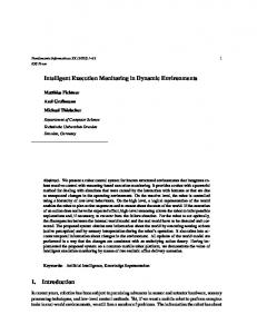
(a) Successful execution of the plan: (1) move (b) During execution of action (1) the exogeto Room A, (2) pick up letter, (3) move to nous event, close door to RoomD , invalidates Room D and (4) release letter. the plan (as the target is not reachable anymore). In (2) the robot detects the closed door and the violation of the plan invariant (accessible(Room D)). Due to the application of plan invariants the infeasibility of the plan is early detected. Fig. 1. Plan execution using plan invariants for the delivery robot example.

In this paper, we present the idea of plan invariants as a means to supervise plan execution. Plan invariants are conditions that have to hold during the whole plan execution. Consider a delivery robot, based on the above architecture. Its task is to transport a letter from room A to room D. This task is depicted in Figure 1. The robot believes that it is located in room C, the letter is in room A and all doors are open. Its goal is that the letter is in room D. The robot might come up with the following plan fulfilling the goal: (1) move to Room A, (2) pick up letter, (3) move to Room D and (4) release letter. In situation (a) no exogenous events occur, the belief of the agent is always consistent with the environment. Therefore, the robot is able to execute the plan and achieves the desired goal. In situation (b) the robot starts to execute the plan with action (1). Unfortunately, somebody closes the door to room D (2). As the robot is not able to open doors, its plan will fail. Without plan invariants the robot will continue to execute the plan until it tries to execute action (3) and detects the infeasible plan. If we use a plan invariant, e.g., room D has to be accessible, the robot detects the violation as it passes the closed door. Therefore, the robot is able to early detect invalid plans and to quickly react to exogenous events.

In the next section we discuss the advantages of plan invariants in more detail. In Section 3 we formally define the planning problem and plan execution. In Section 4 we formally introduce plan invariants. Finally, we discuss related research and conclude the paper.

2 Plan Invariants Invariants are facts that hold in the initial and all subsequent states. Their truth value is not changed by executing actions. There is a clear distinction between these plan invariants to action preconditions, plan preconditions and invariants applied to the plan creation process. Action preconditions have to be true in order to start execution of an action. They are only checked once at the beginning of an action. Similarly, plan preconditions (i.e., initial state) are only checked at the beginning of plan execution. Thus, preconditions reflect conditions for points in time whereas invariants monitor time periods. In the past, invariants have been used to increase the speed of planning algorithms by reducing the number of reachable states. (e.g. [2]). An invariant as previously described characterizes the set of reachable states of the planning problem. A state that violates the invariant cannot possibly be reached from the initial state. For example, this has been efficiently applied to Graphplan [3] as described in [4, 5]. Such invariants can be automatically synthesized as has been shown in [6, 7]. However, plan invariants are not only useful at plan creation time but also especially at plan execution time. To our best knowledge plan invariants have never been used to control plan execution. There is a clear need for monitoring plan execution, because execution can fail for several reasons. Plan invariants can aid in early detection of inexecutable actions, unreachable goals or infeasible actions. .

3 Basic Definitions ACTION a ACTION a

AGENT

AGENT Si

S i+1

Si

STATE

S i+1

Sk

S k+1

ti

STATE TIME

TIME

ENVIRONMENT

(a) Discrete actions

ti

tk

ENVIRONMENT

(b) Durative actions

Fig. 2. Action execution with respect to time

Throughout this paper we use the following definitions which mainly origin from STRIPS planning [1]. A planning problem is a triple (I, G, A), where I is the initial

state, G is the goal state, and A is a set of actions. A state itself is a set of ground literals, i.e., a variable-free predicate or its negation. Each action a ∈ A has an associated precondition pre(a) and effect eff (a) and is able to change a state via its execution. The pre-conditions and effects are assumed to be sets of ground literals. Execution of an action a is started if its pre-conditions are fulfilled in the current state S. After the execution all literals of the action’s effect are elements of the next state S 0 together with the elements of S that are not influenced by action a. A plan p is a sequence of actions < a1 , . . . , an >, that when executed starting with the initial state I results in goal state G. For the delivery example the planning problem is defined as follows. The set of actions is A=< move, pickup, release > with: move(origin, dest): pre: accessible(dest) ∧ isat(R,origin) ∧ ¬ isat(R,dest) eff: ¬ isat(R,origin) ∧ isat(R,dest) pickup(item): pre: isat(R,item) ∧ ¬ hold(item) eff: hold(item) release(item): pre: hold(item) eff: ¬ hold(item) The initial state is I:= isat(letter, Room A) ∧ isat(R,Room C) and the goal is defined as G:= isat(letter, Room D). As the names of constants and predicate are chosen quite intuitively, definitions are omitted due to space limitations. A plan can be automatically derived from a planning problem and there are various algorithms available for this purpose. Refer to [8] for an overview. For the delivery example a planner might come up with the plan p=. The planning problem makes some implicit assumptions for plan computation. First, it is assumed that all actions are atomic and cannot be interrupted. Second, the effect of an action is guaranteed to be established after its execution. Third, there are no external events that can change a state. Only actions performed by the agent alter states. Finally, it is assumed that the time granularity is discrete. Hence, time advances only at some points in time but not continuously. In the most simple way plan execution is done by executing each action of the plan step by step without considering problems that may arise, e.g., a failing action or external events that cause changes to the environment. Formally, this simple plan execution semantics is given as follows (where J K denotes the interpretation function): J< a1 , . .½ . , an >K S = J< a2 , . . . , an >K (Ja1 K S) eff (a) ∪ {x|x ∈ S ∧ ¬x 6∈ eff (a)} if pre(a) ⊆ S JaK S = fail if pre(a) 6⊆ S JaK fail = fail Given the semantics definition of plan execution we can now state what a feasible plan is. Definition 1. A plan p =< a1 , . . . , an > |ai ∈ A is a feasible plan for a planning problem (I, G, A) iff JpK I 6= fail and JpK I ⊇ G.

Planning algorithms always return feasible plans. However, feasibility is only a necessary condition for a plan to be successfully executed in a real environment. Reasons for a plan to fail are: 1. An action cannot be executed. (a) An external event changes the state so that the pre-condition cannot be ensured. (b) The action itself fails because of an internal event, e.g., a broken part. 2. An external event changes the state of the world in a way so that the original goal cannot be reached anymore. 3. The action fails to establish the effect. In order to formalize a plan execution in the real world, we assume the following situation. A plan is executed by an agent/robot which has its view of the world. The agent can modify the state of the world via actions and perceives the state of the surrounding environment via sensors. The agent assumes that the sensor input is reliable, i.e., the perceived information reflects the real state of the world. Hence, during plan execution the effects of the executed actions can be checked via the sensor inputs. For this purpose we assume a global function obs(t) which maps a point in time t to the observed state. Note that we use the closed world assumption. Any predicate remains false until it is observed as true. In order to define the execution of an action in the real world two cases need to be distinguished. Actions can last a fixed, known time. In this case, execution is considered done after that time has elapsed. On the other hand, actions can continue indefinitely, e.g., a move action in a dynamic environment can take unexpectedly long if changes in the dynamic environment require detours. Execution of such an action is considered to be finished as soon as its effect is fulfilled. Following the nomenclature previously used in [9], actions with fixed duration are called discrete, and indefinitely continued actions are called durative. Figure 2 depicts the action execution with respect to time. A discrete action a is executable if its precondition pre(a) is satisfied in state Si , where a state Si = Si−1 ⊕ obs(ti−1 ). The function S ⊕ obs(t) = obs(t) ∪ {l|l ∈ S ∧ ¬l ∈ / obs(t)} defines an update function for the agent’s belief. The function returns all information about the current state that is available, i.e., the observations together with derived conditions during plan execution which are not contradicting the given observations. An action lasts for a given time and tries to establish its effect eff (a) in the succeeding state Si+1 . A durative action a is also executable if its precondition pre(a) is satisfied in state Si . In contrast to discrete actions a durative action a is executed until its effect eff (a) is established in some following state Sk+1 . At each time step tj , i ≤ j ≤ k + 1 a new observation is available, a new state Sj is derived Sj = Sj−1 ⊕ obs(tj−1 ). For each state Sj the condition eff (a) ⊆ Sj is evaluated. A durative action can possibly last forever if it is impossible to establish the effect eff (a). if discrete(a) then JaK (S) =  S ⊕ obs(t) if eff (a) ⊆ (S ⊕ obs(t))  = JexecK(a, S ⊕ obs(t)) if pre(a) ⊆ (S ⊕ obs(t)) ∧ eff (a) 6⊆ (S ⊕ obs(t))  fail otherwise

(1)

In the above definition of the plan execution semantics for single actions we can distinguish three cases. The first line of the definition handles the case where the effect is fulfilled without the requirement of executing the action a. In the second line, the action a is executed which is represented by the exec(a, S) function.  

½ ¯ ¾ ¯ x ∈ (S ⊕ obs(t) ∧ eff (a) ∪ x ¯¯ if action a is executed ¬x 6∈ eff (a) JexecK (a, S) = (2)  fail otherwise

exec(a, S) returns fail if the action a was not executable by the agent/robot in state S. If action a is executed exec returns the effect of the action eff (a) unified with all literals of state S not negated by eff (a). t is the time after executing the action. The last line of the execution semantics states that it returns fail if the precondition of the action is not fulfilled. The action release is an example for a discrete action. Once the action is triggered it either takes a certain amount of time to complete or it fails. For durative actions, execution semantics can be written as follows: S ⊕ obs(t) if eff (a) ⊆ (S ⊕ obs(t)) JaK0 (S ⊕ obs(t)) if pre(a) ⊆ (S ⊕ obs(t)) ∧ if durative(a) then JaK (S) = eff (a) 6⊆ (S ⊕ obs(t))    fail otherwise    

(3)

with

0

JaK (S) =

½

S ⊕ obs(t) if eff (a) ⊆ (S ⊕ obs(t)) JaK0 (S ⊕ obs(t)) otherwise

(4)

The precondition of a durative action is checked only at the beginning of the action. We assume that one recursion of an durative action (equation 4) lasts for a time span greater than zero. The action move is an example for a durative action, as it executed until the robot reaches its destination. This may take different amounts of time or possibly may never occur. Given a plan and a real-world environment we can now define what it means to be able to reach a goal after executing a plan. Definition 2. A plan p =< a1 , . . . , an > for a given planning problem (I, G, A) is successfully executed in a given environment if J< a1 , . . . , an >K(I) ⊇ G.

4 Extended Planning Problem As outlined in Section 2, plan invariants are a useful extension to the planning problem. The addition of an invariant to a planning problem results in the following definition: Definition 3 (Extended Planning Problem). An extended planning problem is a tuple (I, G, A, inv) where inv is a logical sentence which states the plan invariant.

A plan p for an extended planning problem is created using any common planning algorithm. We call the tuple (p, inv) extended plan. The plan invariant has to be fulfilled until the execution of the plan is finished (either by returning the goal state or fail). A plan invariant is a more general condition for feasible plans. It allows for considering exogenous events and problems that may occur during execution, e.g., failed actions. Automatic generation of such invariants is questionable. Invariants represent knowledge that is not implicitly contained in the planning problem, and thus cannot be automatically extracted from preconditions and effect descriptions. An open question is how more knowledge about the environment (e.g., modeling physical laws or the behavior of other agents) and an improved knowledge representation would enable automatic generation of plan invariants. The execution semantics of such an extended plan can be stated using k to denote parallel execution: J(p, inv)K (S) = JpK (S)kJinvK (S)

(5)

Communication between statements executed in parallel is performed through obs, S and the state of plan execution. The semantics of checking the invariant over time is defined as follows:

JinvK(S) =

½

JinvK(S) if inv ∪ (S ⊕ obs(t)) 6|= ⊥ fail otherwise

(6)

where S is the current belief state of the agent and obs(t) results in a set of observations at a specific point in time t. Hence, the invariant is always checked unless it contradicts the state of the world obs or the agent’s belief S. For the delivery example inv = accessible(Room D) ∧ (accessible(Room A) ∨ hold(letter)) would be a feasible invariant. The invariant states that as long as the robot does not hold the letter Room A has to be accessible. Room D has to be accessible during the whole plan execution. Definition 4. An extended plan p = (< a1 , . . . , an >, inv) is a feasible extended plan for a planning problem (I, G, A) iff JpK I 6= fail and JpK I ⊇ G, and all states that are passed by the plan the invariant must hold, i.e., ∀ni=0 (Ja1 , . . . , ai K(I) ∪ inv) 6|= ⊥. Feasibility is again a necessary condition for extended plans to be executable. Hence, it must be guaranteed that the invariant does not contradict any state that is reached during plan execution. We now can easily extend Definition 2 for extended plans. Definition 5. An extended plan p = (< a1 , . . . , an >, inv) for a given planning problem (I, G, A) is successfully executed in a given environment if J(< a1 , . . . , an > , inv)K(I) ⊇ G. Theorem 1. An extended plan p = (< a1 , . . . , an >, inv) for a planning problem (I, G, A) is successfully executed in a given environment with observations obs if (1) the plan is feasible , (2) ∀ni=0 (Ja1 , . . . , ai K(I) ∪ inv) 6|= ⊥. and (3) the set of believed facts resulting from execution of plan p with simple plan execution semantics is a subset of the set of believed facts resulting from execution in a real-world environment.

Regarding Theorem 1 (3), in real-world environments, observations lead to believed facts that are not predictable from the plan execution, hence JaK(S) differs. Corollary 1. Every feasible extended plan for a planning problem (I, G, A) is a feasible plan for the same planning problem. Concluding the execution of a plan does not relieve an agent of its duties. If the plan execution succeeds, a new objective can be considered. If plan execution fails, alternative designations need to be aimed at. Not all possible goals might be desirable, we therefore need a condition that decides about execution. This condition needs to be valid from the beginning of plan creation to the initiation of plan execution, hence the initial state I needs to fulfill this condition, the plan problem precondition. An agent is given a set of alternative planning problems P1 , . . . , Pn and nondeterministically picks one out of these that has a satisfied precondition Ci thus deriving an extended planning problem (I, Gi , A, inv).    C1 → (I, G1 , A, inv)  . Π = ...   Cn → (I, Gn , A, inv)

(7)

The knowledge base of an agent Π comprises all desired reactions of the agent to a given situation. The preconditions trigger sets of objectives the agent may pursuit in the given situation. The execution semantics of this set of planning problems can be stated as follows: JΠK (I) = do for ever select (I, Gi , A, inv) when S |= Ci pi = generate plan(I, Gi , A, inv) J(pi , invi )K (S) end do; The function generate plan generates a feasible plan. The plan could be generated by using any planning algorithm. The use of pre-coded plans is also conceivable. The function select nondeterministically selects one planning problem of the set of planning problems whose precondition is fulfilled. A heuristic implementation of the function is conceivable, if some measure of the performance/quality of the different planning problems is available.

5 Related Research Invariants for planning problems have previously been investigated within the context of planning domain analysis. Planning domain descriptions implicitly contain structural features that can be used by planners while not being stated explicitly by the domain designer. These features can be used to speed up planning. For example, Kautz and Selman [10] used hand-coded invariants provided as part of the domain description used by

Black-box, as did McCluskey and Porteous [11]. The use of such constraints has been demonstrated to have a significant impact on planning efficiency[12]. Such invariants can be automatically synthesized as has been shown in [6, 7, 4]. Even temporal features of a planning domain can be extracted by combining domain analysis techniques and model checking in order to improve planning performance [13]. Also noteworthy is Discoplan [14], a system that uses domain description in PDDL [15] or UCPOP [16] syntax to extract various kinds of state constraints that can then be used to speed up planning. Any forward- or backward-chaining planning algorithm can be enhanced by applying such constraints, e.g. Graphplan [3], as described in [5]. However, in [17] Baioletti, Marcugini and Milani suggest that such a constrained planning problem can be transformed to a non-constrained planning problem, which allows the application of any common planning algorithm. Dijkstra introduced in [18] the concept of guarded commands by using invariants for statements in program languages. This concept is similar to our proposed method except that we use it for plan execution.

6 Conclusion In this article we have presented a framework for executing plans in a dynamic environment. We have implemented the framework in our autonomous robotic platform [19]. The framework is a three-tier architecture which top layer comprises the planner and the plan executor. We use the implementation on our robots in the RoboCup robotic soccer domain which led to promising results. We have further discussed the operational semantics of the framework and have shown under which circumstances the framework represents a language for representing the knowledge of an agent/robot that interacts with a dynamic environment but follows given goals. A major objective of the article is the introduction of plan invariants which allow for representing knowledge that can hardly be formalized in the original STRIPS framework. Summarizing, the main advantages gained by the use of plan invariants are: Early recognition of plan failure - the success of an agent in a environment is crucially influenced by its ability to quickly react to changes that influence its plans. Long-term goals - plan invariants can be used to verify a plan when pursuing long term goals, as the plan’s suitability is permanently monitored. Conditions not influenced by the agent - plan invariants can be used to monitor conditions that are independent of the agent. Such conditions are not appropriate within action preconditions. Exogenous events - it is usually not feasible to model all exogenous actions that could occur, but plan invariants can be used to monitor significant changes that have an impact on the agent’s plan. Intuitive way to represent and code knowledge - as the agent’s knowledge commonly has to be defined manually it is helpful to think of plan preconditions (the situation that triggers the plan execution) and plan invariants (the condition that has to stay true at all times of plan execution) as two distinct matters. Durative actions - plan invariants can be used to detect invalid or unsuitable plans during execution of durative actions. Durative actions, as opposed to discrete actions, can continue indefinitely. Again, plan invariants offer a convenient solution.

References 1. Richard E. Fikes and Nils J. Nilsson. STRIPS: A New Approach to the Application of Theorem Proving to Problem Solving. Artificial Intelligence, 2:189–208, 1971. 2. Jussi Rintanen and J¨org Hoffmann. An overview of recent algorithms for AI planning. KI, 15(2):5–11, 2001. 3. Avrim Blum and Merrick Furst. Fast planning through planning graph analysis. In Proceedings of the 14th International Joint Conference on Artificial Intelligence (IJCAI 95), pages 1636–1642, 1995. 4. M. Fox and D. Long. The automatic inference of state invariants in tim. Journal of Articial Intelligence Research, 9:367–421, 1998. 5. Maria Fox and Derek Long. Utilizing automatically inferred invariants in graph construction and search. In Artificial Intelligence Planning Systems, pages 102–111, 2000. 6. Jussi Rintanen. An iterative algorithm for synthesizing invariants. In AAAI/IAAI, pages 806–811, 2000. 7. G. Kelleher and A. G. Cohn. Automatically synthesising domain constraints from operator descriptions. In Bernd Neumann, editor, Proceedings of the 10th European Conference on Artificial Intelligence, pages 653–655, Vienna, August 1992. John Wiley and Sons. 8. Daniel S. Weld. Recent advances in ai planning. AI Magazine, 20(2):93–123, 1999. 9. Nils J. Nilsson. Teleo-reactive programs for agent control. Journal of Artificial Intelligence Research, 1:139–158, 1994. 10. Henry A. Kautz and Bart Selman. The role of domain-specific knowledge in the planning as satisfiability framework. In Artificial Intelligence Planning Systems, pages 181–189, 1998. 11. T. L. McCluskey and J. M. Porteous. Engineering and compiling planning domain models to promote validity and efficiency. Artificial Intelligence, 95(1):1–65, 1997. 12. Alfonso Gerevini and Lenhart K. Schubert. Inferring state constraints for domainindependent planning. In AAAI/IAAI, pages 905–912, 1998. 13. Maria Fox, Derek Long, Steven Bradley, and James McKinna. Using model checking for pre-planning analysis. In AAAI Spring Symposium Model-Based Validation of Intelligence, pages 23–31. AAAI Press, 2001. 14. Alfonso Gerevini and Lenhart K. Schubert. Discovering state constraints in DISCOPLAN: Some new results. In AAAI/IAAI, pages 761–767, 2000. 15. Maria Fox and Derek Long. PDDL2.1: An Extension to PDDL for Expressing Temporal Planning Domains. University of Durham, UK, 2003. 16. J. Scott Penberthy and Daniel S. Weld. UCPOP: A sound, complete, partial order planner for ADL. In Bernhard Nebel, Charles Rich, and William Swartout, editors, KR’92. Principles of Knowledge Representation and Reasoning: Proceedings of the Third International Conference, pages 103–114. Morgan Kaufmann, San Mateo, California, 1992. 17. M. Baioletti, S. Marcugini, and A. Milani. Encoding planning constraints into partial order planning domains. In Anthony G. Cohn, Lenhart Schubert, and Stuart C. Shapiro, editors, KR’98: Principles of Knowledge Representation and Reasoning, pages 608–616. Morgan Kaufmann, San Francisco, California, 1998. 18. Edsger W. Dijkstra. A Discipline of Programming. Series in Automatic Computation. Prentice-Hall, 1976. 19. Gordon Fraser, Gerald Steinbauer, and Franz Wotawa. A modular architecture for a multipurpose mobile robot. In Innovations in Applied Artificial Intelligence, 17th Conference on Industrial and Engineering Applications of Artificial Intelligence and Expert Systems, IEA/AIE, volume 3029 of Lecture Notes in Artificial Intelligence, Ottawa, 2004. Springer.