Congress on Evolutionary Computation (CEC), Oregon, USA, 2004: 2017-2022
Optimizing Semiconductor Devices by Self-organizing Particle Swarm Xiao-Feng Xie Institute of Microelectronics, Tsinghua University, Beijing 100084, P. R. China Email:
[email protected]
Wen-Jun Zhang Institute of Microelectronics, Tsinghua University, Beijing 100084, P. R. China Email:
[email protected]
Abstract- A self-organizing particle swarm is presented. It works in dissipative state by employing the small inertia weight, according to experimental analysis on a simplified model, which with fast convergence. Then by recognizing and replacing inactive particles according to the process deviation information of device parameters, the fluctuation is introduced so as to driving the irreversible evolution process with better fitness. The testing on benchmark functions and an application example for device optimization with designed fitness function indicates it improves the performance effectively.
I. INTRODUCTION From the deep sub-micrometer to nanoscale devices, the technology CAD (TCAD) tools provide a better insight than measurement techniques and have become indispensable in the new device creation [4]. Technology development, however, requires substantially more than fundamental simulation capability: tools and methods to assist in exploration of design trade-offs and to optimize a design, are becoming increasingly important [6]. As the first step in technology synthesis [6, 8], device optimization problem is to finding some feasible device designables in the design space (S) in order to satisfying the requirements on the device electrical performance. G Each device designable x = ( x1 ,..., xd ,..., xD ) ∈ S is a possible combination of device parameters (xd) that specify the device topography and channel impurity concentrations associated with a semiconductor device. Typical device designables are physical gate length, oxide thickness, etc. The D-dimensional design space (S) is a Cartesian product of domains of device parameters. Device performance is evaluated from the electrical responses of the device. Examples are on and off currents, threshold voltage, output resistance, etc. for MOS devices. For short channel MOS devices, the response surfaces of device performance are often highly nonlinearly. For scaled devices, such surfaces can be even highly rugged due to the disturbance from the mesh adjustment of device simulations, such as PISCES [22]. Moreover, the highly sophisticated novel semiconductor devices involve many design parameters, which increase the dimension of design space. For handling with such complex cases, the global search techniques, such as genetic algorithm (GA) [10], particle swarm optimization (PSO) [5, 7], etc., had been employed in a modeling and optimization system [21] for finding the feasible devices.
De-Chun Bi Department of Environmental Engineering, Liaoning University of Petroleum & Chemical Technology Fushun, Liaoning, 113008, P. R. China
The number of evaluation times is crucially for device optimization since each device simulation is timeconsumptively. As a novel stochastic algorithm, PSO [5, 7] is inspired by social behavior of swarms. Studies [1] showed that although PSO discovered reasonable quality solutions much faster than other evolutionary algorithms (EAs), however, it did not possess the ability to improve upon the quality of the solutions as evolution goes on. Structures of increasing complexity in self-organizing dissipative systems based on energy exchanges with the environment were developed into a general concept of dissipative structures (DS) by Prigogine [10, 12], which allows adaptation to the prevailing environment with extraordinarily flexible and robust. The self-organization of DS was implemented in a dissipative PSO (DPSO) model [19] with some good results. However, the DPSO model also introduces additional control parameters to be adjusted by hand, which cannot be very easily determined. In this paper, the particle swarm is worked in dissipative state with the control parameters according to the experimental convergence analysis results from a simplified model. Instead of introducing additional parameters, the process deviations of device parameters are employed for recognizing inactive particles. Then the negative entropy is introduced to stimulate the model of PSO operating as a DS, which is realized by replacing inactive particles with fresh particles. The variant of particle swarm, termed self-organizing PSO (SOPSO), removes the additional parameters. The performance of the self-organizing PSO is studied on three benchmark functions and an application for a Focused-Ion-Beamed MOSFET (FIBMOS) [13] with designed fitness function, by comparing with some existing algorithms [9, 14, 19]. II. PARTICLE SWARM OPTIMIZATION In particle swarm, The location of the ith ( 1 ≤ i ≤ N , i ∈ ] ) particle is a potential solution in S represented as G xi = ( xi1 ,..., xid ,..., xiD ) . The best previous position (with the best fitness value) of the ith particle is recorded and G represented as pi =(pi1,…, pid, …, piD), which is also called pbest. The index of the best pbest among all the G G particles is represented by the symbol g. The p g (or g ) is also called gbest. The velocity for the ith particle is G vi =(vi1,…, vid, …, viD). At each time step, the ith particle is manipulated according to the following equations [14]:
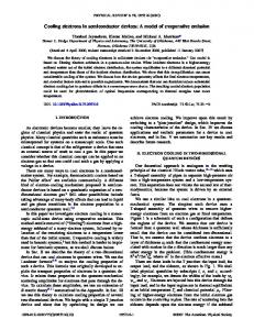
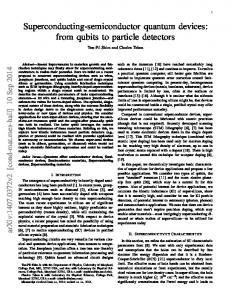
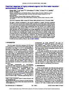
III. EXPERIMENTAL CONVERGENCE ANALYSIS The convergence analysis can be done on a single dimension without loss of generality since there is no interaction between the different dimensions in equations (1), so that the subscript d is dropped. And the analysis is simplified even more for a single particle, then the subscript i is dropped, i.e., (2a) v=w·v+c1· U \ ()·(p-x)+c2· U \ ()·(g-x) x=x+v (2b) Here just consider a special case |p-g|→0, which can be encountered by every particle. By transforming the coordinate origin to g, i.e. p≈g=0, equation (2a) can be simplified as: v=w·v-C·x (3) where C=(c1· U \ ()+c2· U \ ()). Several researchers have analyzed theoretically for the cases when C is fixed [2, 16, 17]. However, it still has great difficulty to analyze the cases when C is stochastically varied. Without loss of generality, here we suppose the g is in a local minimum, i.e. is not changed in the following generations. Fig. 1 gives the average log(|x|) value of 1E6 experimental trails in 100 generations, where log() is the logarithmic operator, the initial x(0) = U \ (), the initial v(0) = U \ (), c1=c2=2. Besides, a special setting that in constriction factor (CF) [2] is also demostrated in Fig.1 as a dash line, which with w=0.729 and c1=c2=1.494. Here it can be seen that the average log(|x|) varied linearly as generation t is increasing. Besides, the CF version lies between w=0.6~0.8 (about 0.65) in the normal version. 8
10
T=100 0 -10 -20 -30 -40 0.0
wth 0.2
0.4
0.6
0.8
1.0
w Figure 2. The average log(|x|) for different w at T=100.
IV. SELF-ORGANIZING PARTICLE SWARM To converge fast with considerable performance, a selforganizing PSO (SOPSO) based on the principle of DS is presented, as shown in Fig. 3.
w=1.0
0
0.8
-8
log(|x|)
and be dissipative state when 0 ≤ w ≤ wth , here wth is about equal to 0.85. Of course, for real swarm, such threshold value should be decreased slightly since normally p ≠ g at the initial time. The value of w that provides balance between exploitation and exploration is lower than the wth, which is about 0.5~0.75 [11, 19], since the performance of swarm decreases when it be too dissipative or be too chaos. Moreover, it can be seen there has a higher tail when w is closed to zero, which is agreed with the increasing fitness at the tail of the experimental results [19] for Rastrigrin and Griewank functions.
log(|x|)
vid=w·vid+c1· U \ ()·(pid-xid)+c2· U \ ()·(gd-xid) (1a) (1b) xid=xid+vid where w is inertia weight, c1 and c2 are acceleration constants, U \ () are random values between 0 and 1.
CF 0.6
-16 -24
0.4 0.0
-32
0.2 0
20
40
60
80
Figure 3. Principle of self-organizing PSO: performing as a DS.
100
t
Figure 1. The average log(|x|) for different w in 100 generations.
Fig. 2 gives the average log(|x|) for different w in T=100 generations. The swarm is in chaotic state when w>wth,
Firstly, as a prerequisite of DS [10, 12], small w, which is much less than wth, is adopted to induce the dissipative processes into the particle swarm, i.e. to reduce the average energy of swarm during evolution according to the nonlinear interactions among particles. Secondly, the self-organization requires a system consisting of multiple elements in which nonlinear interactions between system elements are present [10]. In PSO, the equation (1) ensures nonlinear relations of positive and negative feedback between particles
according to the cooperation and competition with the particle with best experience so far. Thirdly, far-from-equilibrium conditions should be taken for granted [12]. As time goes on, some particles become inactive [20] when they are similar to the gbest and lost their velocities, which lost both of the global and local search capability in the next generations. Since the inactive particle has less contribution on evolution results, it suggests an adaptive mechanism to introduce negative entropy as following: recognize and replace it. Taking the problem information into account can improve the algorithm performance [18]. For each device, there exists process deviation σ d for each parameter xd. G For a given point o , its similar set Ss is defined as all the points within the range of the deviations. Then for G ∀x ∈ S s , which |xd-od| ≤ σ d come into existence in all
G
G
G
G
dimensions, is noted as x ≅ o , i.e. x is similar to o . Then a particle can be identified as inactive if it is always G flying in Ss of p g and without any improvement on its fitness in the following Tc generations. The pseudo code for recognizing inactive particle is shown in Fig. 4, which is executed after equations (1). The SC array is employed to store the times that are similar to the gbest in successively for each particle. Tc is a predefined constant. It need not be too large since the swarm dynamics is dissipative. According to our experience, Tc=2 is good enough.
G
IF ( xi
G ≅ g && i!=g)
THEN SC[i] ++;
// similar to the gbest? // increase 1
ELSE SC[i] = 0;
// reset to 0
IF (SC[i]>Tc)
// achieve predefined count?
THEN the ith particle is inactive;
G
The total fitness function F ( x ) is defined as: G G G F ( x ) =< FOBJ ( x ), FCON ( x ) >
(5)
m G G G G where FOBJ ( x ) = ∑ w j f j ( x ) and FCON ( x ) = ∑ Gk ( x) are
m0
j =1
k = m0 +1
the fitness functions for objectives and constraints, respectively, where wj are positive weight constants, which default values are equal to 1, and G 0 g k ( x ) ∈ [cl , k , cu , k ] G G G (6) Gk ( x ) = (cl , k − g k ( x )) Ak g k ( x ) < cl , k G G > ( ) g x c − ( ( ) ) g x c B k u,k u,k k k | c | c ≠ 0 | c u , k | cu , k ≠ 0 l , k l,k where Ak = and Bk = are cl , k = 0 cu , k = 0 1 1 used for normalizing the large differences in the magnitude of the constraint values for device performance. In order to avoid the difficulty to adjusting penalty coefficient in penalty function methods [9], the fitness evaluation is realized by directly comparison between any G G G G two points x A , xB , i.e. F ( x A ) ≤ F ( xB ) when G G FCON ( x A ) < FCON ( xB ) OR (7) G G G G FOBJ ( x A ) ≤ FOBJ ( xB ), FCON ( x A ) = FCON ( xB ) G If FCON =0, then x ∈ S F . It is also following the Deb’s G G criteria [3]: a) any x ∈ S F is preferred to any x ∉ S F ; b) among two feasible solutions, the one having better FOBJ is preferred; c) among two infeasible solutions, the one having smaller FCON is preferred. The device simulator may also be failed to calculate the responses for some designables when meets with inappropriate mesh settings. Then for such wrong cases, FOBJ = FCON =+∞. VI. RESULTS AND DISCUSSION
Figure 4. Pseudo code for recognizing an inactive particle.
A. Benchmark functions If the ith particle is recognized as inactive, then it is G G replaced by a fresh particle, which the location xi and vi is reinitialized at random, and SC[i] is reset to 0. V. FITNESS FUNCTION DESIGN Typical requirements on device responses are classified in two classes of objectives: G (MIN type) minimize : f j ( x ), for j ∈ [1, m 0 ] (4) G g ( x ) ∈ [ c , c ], for k ∈ [ m + 1, m ] (CON type) k l ,k u,k 0
where f and g are response functions calculated by device simulator. The number of functions in MIN type often are normally 0 or 1 [8, 21]. The set of points, which satisfying all functions gk in CON type, is denoted as feasible space (SF).
For comparison, three unconstrained benchmark functions that are commonly used in the evolutionary computation literature [14] are used. It can be done loss of G generality, since the F ( x ) of constrained function can be seemed as a uncostrained function. All functions have same minimum value, which are equal to zero. The function f1 is the Rosenbrock function: G D −1 f1 ( x ) = ∑ (100( xd +1 − xd2 ) 2 + ( xd − 1) 2 ) (8a) d =1
The function f2 is the generalized Rastrigrin function: D G (8b) f 2 ( x ) = ∑ ( xd2 − 10cos(2π xd ) + 10) d =1
The function f3 is the generalized Griewank function: 1 D 2 D G x (8c) f3 ( x ) = ∑ xd − ∏ cos d + 1 d =1 4000 d =1 d
For dth dimension, xmax,d=100 for f1, xmax,d=10 for f2; xmax,d=600 for f3. Acceleration constants c1=c2=2. The fitness value is set as function value. We had 500 trial runs for every instance. Table 1 lists the initialization ranges. Table 2 gives the additional test conditions. FPSO give the results of fuzzy adaptive PSO [14]. DPSO give the results of PSO version in, which cv=0, cl=0.001 [19]. For SOPSO, w=0.4, and σd=0.01 for the dth dimension of all functions. In order to investigate whether the SOPSO scales well or not, different numbers of particles (N) are used for each function which different dimensions. The numbers of particles N are 20, 40 and 80. The maximum generations T is set as 1000, 1500 and 2000 generations corresponding to the dimensions 10, 20 and 30, respectively. TABLE 1. INITIALIZATION RANGES Function Asymmetric Symmetric f1 (15,30) (-100, 100) f2 (2.56,5.12) (-10,10) (300,600) (-600,600) f3
TABLE 5. THE MEAN FITNESS VALUES FOR THE GRIEWANK FUNCTION N
D
T
FPSO [14]
DPSO[19]
20
10
1000
0.091623
0.06506
SOPSO 0.06100
20
1500
0.027275
0.02215
0.02365
30
2000
0.02156
0.01793
0.02326
10
1000
0.075674
0.05673
0.05251
20
1500
0.031232
0.02150
0.01783
40
80
30
2000
0.012198
0.01356
0.01271
10
1000
0.068323
0.05266
0.04659
20
1500
0.025956
0.02029
0.01932
0.01190
0.01034
30
2000
0.014945
Table 3 to 5 lists the mean fitness values for three functions. It is easy to see that SOPSO have better results than FPSO [14] for almost all cases. By compare it with the results of DPSO [15], SOPSO also performs better for all the cases of Rosenbrock function, and better than most cases of Griewank function slightly, although it performs worse for the cases of Rastrigrin function.
TABLE 2. TEST CONDITIONS FOR DIFFERENT PSO VERSIONS PSO Type FPSO [14] DPSO [19] SOPSO
B. Device Optimization Example
Initialization w
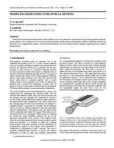
The performance of SOPSO was also demonstrated on a double-implantation focused-ion-beam MOSFETs [13, 21], as shown in Fig. 5. A device simulator PISCES-2ET [22] is used to calculate the device characteristics. Here most parameters are fixed. The effective channel length (Leff) is 0.25µm; the oxide thickness (Tox) is 0.01µm. For source and drain, the junction depth (Xj) is 0.1µm, doping concentration (NSD) is 7.0E20cm-3. For both of the P+ implant peaks in the channel, there have same implant energy as 10keV.
Asymmetric Fuzzy
Symmetric 0.4
Symmetric 0.4
TABLE 3. THE MEAN FITNESS VALUES FOR THE ROSENBROCK FUNCTION N
D
T
FPSO [14]
DPSO
20
10
1000
66.01409
35.7352
20
1500
108.2865
78.5368
47.1619
40
80
SOPSO 21.7764
30
2000
183.8037
132.1512
72.1907
10
1000
48.76523
17.0553
13.4052
20
1500
63.88408
43.8963
29.2476
30
2000
175.0093
82.7209
52.2661
10
1000
15.81645
17.7516
11.9570
20
1500
45.99998
32.2961
26.5855
30
2000
124.4184
57.2802
46.9986
TABLE 4. THE MEAN FITNESS VALUES FOR THE RASTRIGRIN FUNCTION D
20
10
1000
20
1500
23.27334
30
2000
48.47555
40
80
T
FPSO [14]
N
4.955165
Tox SOURCE N+
0
P+
Dose1
P+
Peak 1
X1
Nsub
GATE
X2
0.25
Peak 2
Xj
DRAIN N+
Dose2
Leff SUBSTRATE
SOPSO 1.0079
Figure 5. Schematic of 0.25µm double-implantation MOS device.
2.5729
6.8493
7.3258
17.7011
TABLE 6. DEVICE SEARCH SPACE AND PARAMETER PRECISIONS Name Min Max σ Unit X1 0.00 0.25 2.5E-4 µm Dose1 1E10 1E13 1E10 cm-2 X2 0.00 0.25 2.5E-4 µm Dose2 1E10 1E13 1E10 cm-2 Nsub 1E15 1E18 1E15 cm-3
DPSO[19] 0.4707
10
1000
3.283368
0.0762
0.1576
20
1500
15.04448
1.3088
3.2670
30
2000
35.20146
6.2107
9.5294
10
1000
2.328207
0.0080
0.0086
20
1500
10.86099
0.7496
1.3517
30
2000
22.52393
4.2265
4.9781
The design parameters include lateral implantation position that start from source side of channel for peak 1
(X1) and 2 (X2), implantation dose in peak 1 (Dose1) and 2 (Dose2), and substrate doping concentration (Nsub). Table 6 lists the lower and upper boundary value and the precision σ for each parameter, which includes almost all the possible implantation states in the device channel. Table 7 lists the objectives, which includes drive current (Ion) and output conductance (Gout) at Vds=1.5V, Vgs=1.5V; and off current (Ioff) at Vds=1.5V and Vgs=0V. TABLE 7. OBJECTIVES: DESIRED DEVICE PERFORMANCE Name Objective Unit Ion maximize A/µm Ioff A/µm ≤ 1E-14 Gout 1/Ω ≤ 8E-6
Several algorithm settings are tested. GENOCOP is a real-value genetic algorithm (GA) with multiply genetic operators [9], which had applied for optimizing device successfully [8, 21]. Here its population size is set as Npop=50. For each generation, it has Nc=10~12 children individuals, the selection pressure q=0.01. For standard PSO, w are fixed as 1 [7], 0.4, and a linearly decreasing w which from 0.9 to 0.4 [14], respectively. For SOPSO, w is fixed as 0.4. The number of particles N=10 for all the PSO versions. We had 20 trial runs for every instance. GENOCOP PSO: w = 1 PSO: w = 0.9->0.4 PSO: w = 0.4 SOPSO: w = 0.4
VII. CONCLUSION In this paper, a self-organizing PSO was presented by simulating the self-organization. The particle swarm is worked in dissipative condition by employing a small w, based on experimental analysis for a simplified model, which with fast convergence. Then the negative entropy is introduced, which is realized by recognizing and replacing inactive particles according to the existing information of the problem, i.e. the process deviations of device parameters, so as to driving the irreversible evolution process with better fitness, while removes the additional control parameters. The testing of three benchmark functions indicates the SOPSO has good performance. Then the testing results on a FIBMOS device illustrate that the SOPSO has fast optimization capability from the early searching stage, which is crucially for device optimization since each evaluation by device simulation is time-consumption. REFERENCES
F∆
1E-5
linearly decreasing w which from 0.9 to 0.4 performed better than the PSO version with w=0.4 at last which converged slowly at the early stage while fastly at the last stage,. Moreover, the SOPSO performed as the best in all cases, which evolving sustainable when the evolution of PSO with same w is going to be stagnated. In addition, SOPSO costed only 24 generations to achieve the performance of GENOCOP, and only 46 generations to achieve the performance of PSO with w =0.4.
[1] Angeline P J. Evolutionary optimization versus particle swarm optimization: philosophy and performance difference. Annual Conf. on Evolutionary Programming, San Diego, CA, USA, 1998: 601-610 Ion,max=1.16411E-4(A/µm)
1E-6 0
20
40
60
80
100
t (generations)
Figure 6. Relative mean fitness F∆ of device optimization results.
Fig. 6 shows the relative mean performance F∆=|FoptFB| during 100 generations for different algorithms. Where FB is the mean fitness value of the best particle found in current generation that found by algorithm, and Fopt=1.16411E-4A/µm is the optimum value for Ion when satisfying the constraints on Ioff and Gout. For all the PSO versions, the total evaluation times is Te=1000, which is a little less than that of GENOCOP (about 1050~1250). It shows that the original PSO version with w=1 [7], performed worst in all cases since it is worked in chaotic state. However, all the other PSO versions perform better than GENOCOP. The PSO version with w=0.4 converged fastly and stagnated at the last stage of evolution, since it is worked in dissipative state. The PSO version with a
[2] Clerc M, Kennedy J. The particle swarm - explosion, stability, and convergence in a multidimensional complex space. IEEE Trans. Evolutionary Computation, 2002, 6(1): 58-73 [3] Deb K. An efficient constraint handling method for genetic algorithms. Computer Methods in Applied Mechanics and Engineering, 2000, 186(2-4): 311-338 [4] Dutton R W, Strojwas A J. Perspectives on technology and technology-driven CAD. IEEE Trans. Computer-aided Design of Integrated Circuits and Systems, 2000, 19(12): 1544-1560 [5] Eberhart R C, Kennedy J. A new optimizer using particle swarm theory. Int. Symposium on Micro Machine and Human Science, Nagoya, Japan, 1995: 39-43 [6] Hosack H H, Mozumder P K, and Pollack G P. Recent advances in process synthesis for semi-conductor devices. IEEE Trans. Electron Devices, 1998, 45 (3): 626 – 633 [7] Kennedy J, Eberhart R. Particle swarm optimization. Proc. IEEE Int. Conf. on Neural Networks, Perth, Australia, 1995: 1942-1948
[8] Li Z, Xie X F, Zhang W J, et al. Realization of semiconductor device synthesis with the parallel genetic algorithm. Asia and South Pacific Design Automation Conference, Yokohama, Japan, 2001: 45-49 [9] Michalewicz Z. Genetic algorithms + Data structures = Evolution programs, Springer-Verlag, Berlin, 1994 [10] Nicolis G, Prigogine I. Self-organization in nonequilibrium systems: from dissipative systems to order through fluctuations, John Wiley, New York, 1977 [11] Parsopoulos K E, Vrahatis M N. Recent approaches to global optimization problems through particle swarm optimization. Natural Computing, 2002 (1): 235-306 [12] Prigogine I. Introduction to thermodynamics of irreversible processes. John Wiley, New York, 1967 [13] Shen C C, Murguia J, Goldsman N, et al. Use of focusedion-beam and modeling to optimize submicron MOSFET characteristics. IEEE Trans. Electron Devices, 1998, 45(2): 453-459 [14] Shi Y H, Eberhart R C. Empirical study of particle swarm optimization. Congress on Evolutionary Computation, Washington DC, USA, 1999: 1945-1950 [15] Shi Y H, Eberhart R C. Fuzzy adaptive particle swarm optimization, IEEE Int. Conf. on Evolutionary Computation, Seoul, Korea, 2001: 101-106 [16] Trelea I C. The particle swarm optimization algorithm: convergence analysis and parameter selection. Information Processing Letters, 2003, 85(6): 317–325 [17] van den Bergh F. An Analysis of Particle Swarm Optimizers, Ph.D thesis, University of Pretoria, South Africa, 2001 [18] Wolpert D H, Macready W G. No free lunch theorems for optimization. IEEE Trans. Evolutionary Computation, 1997, 1(1): 67-82 [19] Xie X F, Zhang W J, Yang Z L. A dissipative particle swarm optimization. Congress on Evolutionary Computation, Honolulu, HI, USA, 2002: 1456-1461 [20] Xie X F, Zhang W J, Yang Z L. Adaptive particle swarm optimization on individual level. Int. Conf. on Signal Processing, Beijing, China, 2002: 1215-1218 [21] Xie X F, Zhang W J, Lu Y, et al. Modeling and optimization system for semiconductor devices. Chinese J. Semiconductors, 2003, 24(3): 327-331 (In Chinese) [22] Yu Z P, Chen D, So L, Dutton R W. PISCES-2ET manual. Integrated Circuits Laboratory, Stanford University, 1994


![RESURF power semiconductor devices[]](https://m.moam.info/img/260x300/resurf-power-semiconductor-devices_5b97e410097c47f9508b46cb.jpg)