Optimizing Top-N Collaborative Filtering via Dynamic Negative Item Sampling Weinan Zhang† , Tianqi Chen‡ , Jun Wang† , Yong Yu‡ †
‡
Dept. of Computer Science, University College London Dept. of Computer Science and Engineering, Shanghai Jiao Tong University
{w.zhang, j.wang}@cs.ucl.ac.uk, {tqchen, yyu}@apex.sjtu.edu.cn ABSTRACT Collaborative filtering techniques rely on aggregated user preference data to make personalized predictions. In many cases, users are reluctant to explicitly express their preferences and many recommender systems have to infer them from implicit user behaviors, such as clicking a link in a webpage or playing a music track. The clicks and the plays are good for indicating the items a user liked (i.e., positive training examples), but the items a user did not like (negative training examples) are not directly observed. Previous approaches either randomly pick negative training samples from unseen items or incorporate some heuristics into the learning model, leading to a biased solution and a prolonged training period. In this paper, we propose to dynamically choose negative training samples from the ranked list produced by the current prediction model and iteratively update our model. The experiments conducted on three large-scale datasets show that our approach not only reduces the training time, but also leads to significant performance gains.
Categories and Subject Descriptors H.3.3 [Information Systems]: Information Search and Retrieval—Information Filtering
General Terms Algorithms, Experimentation
Keywords Ranking-Oriented Collaborative Filtering, Recommender Systems, Negative Item Sampling
1.
INTRODUCTION
Recommender systems have been widely used in various Internet services. Collaborative Filtering (CF) is one of the most widely used techniques for recommender systems. It leverages the user-item preference (or rating) patterns derived from a large amount of historic data to make the recommendation. Different recommendation scenarios could result in different CF models. Top-N recommendation is Permission to make digital or hard copies of all or part of this work for personal or classroom use is granted without fee provided that copies are not made or distributed for profit or commercial advantage and that copies bear this notice and the full citation on the first page. Copyrights for components of this work owned by others than ACM must be honored. Abstracting with credit is permitted. To copy otherwise, or republish, to post on servers or to redistribute to lists, requires prior specific permission and/or a fee. Request permissions from
[email protected]. SIGIR’13, July 28–August 1, 2013, Dublin, Ireland. Copyright 2013 ACM 978-1-4503-2034-4/13/07 ...$15.00.
one of the most common scenarios, where it delivers a topN ranked list of the most relevant items to the user for each recommendation interaction. Thus the goal of top-N CF modelling is to produce an optimal item rank function given a user profile [2]. As the rankings of the top items are more important than lower ones, which is consistent with the users’ top-down browsing behaviors, similar to the Learning to Rank problem in text retrieval, rank biased performance evaluation measures, such as NDCG and MAP, have been used to evaluate the performance of top-N recommendation. However, there is a significant difference between CF and text retrieval. There has been a large body of research on ranking-oriented CF. Most solutions rely on pair-wise comparison. Generally speaking, pair-wise CF approaches first sample some positive-negative item pairs for each user, and then train the model parameters with the target of correctly identifying the positive/negative item in each pair [5]. Different from the Learning to Rank problem in text retrieval, where a candidate set of documents has been given by the retrieval module, for ranking-oriented CF on implicit user feedback there are always a huge number of unobserved items (which the target user has not rated or clicked) to be considered. Thus there is a significant need for sampling negative items from the unseen samples in the collection1 . For example, for each item with positive feedback, a number (usually between 1 and 5) of the unobserved items are randomly sampled to act as the negative ones in the training data of the pair-wise ranking model. In addition to the pair-wise CF approaches, the list-wise approaches inspired by Learning to Rank techniques for text retrieval have also been introduced (e.g., [8]). However, due to their difficulty in modeling the inter-list loss and inefficiency on large scale datasets, list-wise CF approaches are not widely used compared to pair-wise in ranking-oriented CF. In this paper, we focus on pair-wise CF approaches using implicit feedback data. A popular pair-wise CF algorithms is Bayesian Personalized Ranking (BPR) [5]. BPR uniformly samples negative items for each positive item and optimizes the AUC measure, which is, unfortunately, not a rank biased performance measure. Therefore, BPR does not distinguish the ranking performance between the items ranked 1st and 1000th. However, as discussed above, the rank biased performance measures such as NDCG and MAP are more suitable as top-N recommendation evaluation measures. Therefore, if we want to optimize such measures, BPR actually performs 1
As a training process, an acceptable target is to rank the observed items (with positive feedback) higher than the unobserved ones for each user, which makes it reasonable to treat the unobserved items as negative samples.
biased training. One intuitive solution to such problem might be adding a learning weight for each pair. However, we argue that such approach is almost useless because randomly picking negative training items among such a huge unobserved item set will make most pairs uniformly low weight. In this paper, we propose dynamic negative item sampling strategies to optimize the rank biased performance measures for top-N CF tasks. We hypothesize that during the training, any unobserved item should not be ranked higher than any observed positive training items because 1) given the fact that the large amount of unseen items in the collection are negative, it is unlikely that an unobserved yet positive item is to be selected from a sampling procedure; and 2) even if it is a positive item, it should not be ranked higher than the known positive ones, as long as it is ranked higher than other unobserved items. Based on our hypothesis, we develop our sampling strategies. Through experiments conducted on three well-known large-scale CF datasets (Netflix, Yahoo! Music, and Last.fm), we discover that choosing unseen items with high ranking score given by the current training model as negative samples will not only significantly improve the rank biased performance measures (effectiveness), but also accelerate the model convergence (efficiency).
2.
PRELIMINARIES
To make this paper self-contained, we first have a brief review on the BPR model and LambdaRank [1] before we present the dynamic negative item sampling strategies in Section 3. First we start from BPR [5]. A basic latent factor model is stated in Eq. (1). rˆui = µ + bu + bi + pTu qi
Du = {hi, jiu |i ∈ Iu ∧ j ∈ I\Iu }, where I represents the whole item set and Iu represents the set of items that user u has given positive feedback. The cost on each item pair hi, jiu is defined using area under ROC curve (AUC) as (2)
where zu is the normalization term and loss function δ(ˆ rui − rˆuj ) can be normally implemented as logistic loss2 , which is always explained as the inverse probability of ranking item i higher than j. δ(ˆ rui − rˆuj ) =
1 1 + erˆui −ˆruj
(3)
The factor in SGD update rule for each parameter w is written as ∂C(hi, jiu ) ∂C(hi, jiu ) ∂(ˆ rui − rˆuj ) = ∂w ∂(ˆ rui − rˆuj ) ∂w ∂ rˆui ∂ rˆuj ≡ λij ( − ), ∂w ∂w
1.
(4)
r ˆui where ∂∂w belongs to the latent factor model parameter updating, and λij can be regarded as the learning weight for this pair. Just like the ranking performance optimization in IR tasks, we can borrow the idea of LambdaRank [1] to 2 In addition, δ(·) can be implemented using other functions such as the 0-1 or hinge loss.
Two example pairs for posive item 6
2. Item Pair :
NDCG = 0.302
Item Pair :
NDCG = 0.035
3. 4. 5. 6. : Unobserved Item
: Posive Item
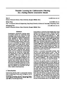
Figure 1: An example rank list produced by the current model. The pair with the item in rank 1 as the negative sample has a higher ∆N DCG weight than the one with item in rank 4 as the negative sample. optimize the rank biased performance measures in top-N CF tasks. We formulate a LambdaRank weight function as f (λij , ζu ), where ζu is the current item ranking list for user u. Thus ∂C(hi, jiu ) ∂ rˆui ∂ rˆuj = f (λij , ζu )( − ), ∂w ∂w ∂w
(5)
where f (λij , ζu ) assigns a learning weight on each BPR pair hi, jiu based on the current item ranking list ζu . By defining different f (λij , ζu ), we can obtain different goals in various item recommendation tasks. In IR tasks with NDCG as target, f (λij , ζu ) can be defined as (in [1]) f (λij , ζu ) ≡ λij ∆N DCGij ,
(1)
As a pair-wise ranking approach, BPR takes each item pair as its training case for each user. The (implicit feedback) training data for user u can be formalized as
C(hi, jiu ) = zu δ(ˆ rui − rˆuj ),
Current Item Ranking List
(6)
where ∆N DCGij is the absolute changed NDCG value for the ranking list ζu if item i and j get switched. This implementation is reasonable in IR but unfortunately impractical in top-N CF tasks. The reason is that to calculate ∆N DCGij of different item pairs, the system needs to rank all the items. In IR tasks, the candidate documents returned by the retrieval model have been limited to a small size (e.g, 1,000). However, in top-N CF tasks, since there is no query at all, all the unobserved items can be regarded as candidates. Thus the ranking list is always large in size (e.g., 624,961 for Yahoo! Music), which makes the ranking process and the calculation of f (λij , ζu ) very time-consuming.
3.
DYNAMIC NEGATIVE ITEM SAMPLING
To solve this problem, we propose a series of negative item sampling strategies. Suppose we have an ideal LambdaRank weight function f (λij , ζu ) for each possible training item pair hi, jiu given the current item ranking list ζu , the main idea is if we have a scheme that generates the training item pair hi, jiu with the probability proportional to f (λij , ζu )/λij (just like ∆N DCGij in the case of Eq. (6)), then we have an almost equivalent training model.
3.1
Rank-aware Reject Sampling Strategies
Figure 1 gives an example of which item pair should have a higher weight. As a general result, the item pairs whose negative item has a higher ranking should be sampled with higher probability. It satisfies regardless of the ranking of the positive item. This is intuitively correct because the higher ranked negative items hurt the ranking performance of the current model more than the lower ranked ones; Even if such unobserved item is a relevant one, ranking it lower
Sampling probability density
Linear
Algorithm 1 Ranking-Aware Reject Sampling - Linear Require: Unobserved item set I\Iu , scoring function s(·), parameter β Draw sample j, l uniformly from I\Iu Query s(j) and s(l) if s(j) > s(l) then 1 , or return l otherwise Return j with probability 1+β else 1 , or return j otherwise Return l with probability 1+β end if
than observed positive items is still reasonable. Thus more training effort should be paid on such pairs. However, an efficiency problem arises as we have to rank all unobserved items. Here we propose a ranking-aware reject sampling algorithm to solve the ranking efficiency problem. We need to draw a sample from the unobserved item set I\Iu , and the probability of picking the item j as the negative item satisfies pj ∝ f (λij , ζu )/λij ≡ g(xj ),
(7)
where g(xj ) is a sampling weight function, and xj ∈ [0, 1] is the relative ranking position of item j in the unobserved item list. Here xj = 0 means ranking at the top and xj = 1 means ranking at the tail. In addition, we suppose that the items are ranked via the scores from a scoring function s(j). Now the goal is to efficiently pick the items at higher rank (with lower xj ) with higher probability.
3.1.1
Linear Weighting Function
We first design the reject sampling procedure in Algorithm 1. Then the probability of item j to be sampled satisfies β 1 Pr(s(j) > s(l)) + Pr(s(j) ≤ s(l)) 1+β 1+β ∝ (1 − xj ) + βxj = −(1 − β)xj + 1 ≡ g(xj ). (8)
pj =
We can find the sampling probability is a linear function to the relative ranking position. Furthermore, the time complexity is O(1), much lower than the brute-force version, which requires O(|I\Iu |) computation time.
3.1.2
General Polynomial Weighting Function
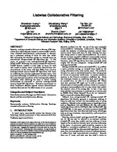
We can generalize the sampling weight function to ndegree polynomial ones with n + 1 samples to be drawn, as shown in Algorithm 2. Then the probability of item j to be sampled satisfies pj ∝ 1Cn0 (1 − xj )n +
n X
βk Cnk xkj (1 − xj )n−k ,
(9)
k=1
which is a polynomial function with degree of n. In particular, setting all βk = 0, we can get a scheme that picks the top from n + 1 randomly selected items, which is O(n + 1) time complexity. Figure 2 gives several examples of sampling weight functions.
3
1.5 2 1 1 0.5 0
0
0.5 Relative ranking
0
1
0
5−Degree Polynomial Sampling probability density
Algorithm 2 Ranking-Aware Reject Sampling - General Require: Unobserved item set I\Iu , scoring function s(·), parameters β1 , β2 . . . , βn Draw sample j1 , . . . , jn+1 uniformly from I\Iu Query s(j1 ), . . . , s(jn+1 ) Sort j1 , . . . , jn+1 by descending order of s(j1 ), . . . , s(jn+1 ) Return one item from the sorted listP with the multinomial distribution {1, β1 , β2 . . . , βn }/(1 + n k=1 βk )
Quadratic
2
0.5 Relative ranking
1
10−Degree Polynomial
6 10 8
4
6 4
2
2 0
0
0.5 Relative ranking
0
1
0
0.5 Relative ranking
1
Figure 2: Illustrations for different sampling weight functions. Here for each function, all βk = 0. Table 1: Characteristics of the datasets. Dataset Users Items Ratings
3.2
Netflix 480,189 17,770 100,480,507
Yahoo! Music 1,000,990 624,961 262,810,175
Last.fm 992 961,417 19,150,868
Relationship with Other Approaches
Due to the page limit, we will not give a general discussion of related works in this paper, but focus on the relationship between our approach and other related ones. So far, we have proposed the dynamic negative item sampling strategies to efficiently optimize the rank biased performance measures for top-N CF tasks. This is essentially different from most ranking-oriented CF algorithms [6, 7, 9] where firstly the target ranking function is somehow smoothed and then a pair-wise or list-wise learning method is performed. Our framework is adaptive to different ranking measures, just by defining different negative item sampling strategies. Compared with LambdaRank [1] in IR tasks, we point out the impractical computation cost problem in topN CF tasks, which makes clear that the dynamic negative item sampling strategy is a key contribution of this work. Among CF works, there are also some negative item sampling considerations but they focus on different performance measures in other CF tasks, such as RMSE in one-class CF [4] and serendipity in music/movie recommendation [3]. In addition, none of these works involves dynamic negative item sampling strategies.
4. 4.1
EXPERIMENTS Experiment Setup
We conduct our experiment on three widely used largescale CF datasets: Netflix, Yahoo! Music, and Last.fm. Details of these three datasets are shown in Table 1. Following the experiment setting of [3], we pick the 5-star ratings for Netflix and 80 or higher ratings for Yahoo! Music as positive feedbacks, and Last.fm itself is an implicit feedback dataset. For training and test data splitting, we follow [3] to use the original splitting on Netflix and Yahoo! Music; and we follow [10] to give a 4:1 random splitting on Last.fm. For comparison, since BPR is a strong baseline and we mainly focus on the impact of dynamic negative item sampling in this paper, here we only compare our approaches with BPR. Both BPR and our approach (denoted as DNS) are built based on SVD as in Eq. (1). Following [3, 10], the factor number of SVD is set to 100. Similar experimental
Table 2: Ranking performance comparison, where “*” means significant improvement.
BPR DNS Impv.
P@5 0.1588 0.4243 167.2%*
BPR DNS Impv.
P@5 0.1231 0.1323 7.5%*
NDCG@10 0.2017 0.2887 43.1%*
MAP 0.1403 0.2036 45.1%*
NDCG@10 0.1481 0.3981 168.8%*
MAP 0.0615 0.1644 167.3%*
NDCG@10 0.1207 0.1250 3.6%
MAP 0.0221 0.0223 0.9%
NDCG
P@5 0.3826 0.4708 23.1%*
0.135
0.4 0.35 NDCG
BPR DNS Impv.
Netflix P@10 NDCG@5 0.3272 0.2052 0.4012 0.2906 22.6%* 41.6%* Yahoo! Music P@10 NDCG@5 0.1359 0.1683 0.3671 0.4458 170.1%* 164.9%* Last.fm P@10 NDCG@5 0.1168 0.1270 0.1202 0.1355 2.9% 6.7%*
Last.fm
Yahoo! Music 0.45
0.3 0.25 NDCG@5 NDCG@10
0.2
0.13 0.125 NDCG@5 NDCG@10
0.12
0.15 0
2
4 6 8 10 Polynomial degree
12
0
5 10 15 Polynomial degree
20
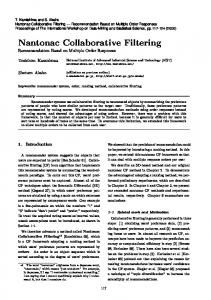
Figure 3: NDCG Performance against polynomial degrees on Yahoo! Music and Last.fm. 0.3
0.25
4.2 4.2.1
Overall Ranking Performance
Convergency and Efficiency
From the time complexity analysis in Section 3.1.2, we know that the time complexity is linear with respect to the polynomial degree of the sampling weight function. However, this fact does not mean the higher-degree sampling weight function is necessarily more inefficient, because it can requires fewer training rounds to get the model converged. In Figure 4, we compare the performance convergence of 3 The popularity-based recommendation generally works worse on more long tailed datasets.
0.2
BPR DNS−Lin DNS−5 DNS−14
0.15
Results and Discussion
First we provide the overall performance of the compared approaches on the three datasets, shown in Table 2. Here the performance of DNS is equipped with the optimal sampling strategy. From the result we can see the significant improvements brought from our approach on almost all the measures and datasets, which shows the effectiveness and robustness of our approach. Furthermore, among the three datasets, the improvement on Yahoo! Music is the most significant and the one on Last.fm is the least. Actually, from the experiment we find the fact that BPR’s recommendation is somehow similar with popularity-based recommendation since it performs the uniform negative item sampling and optimizes AUC. This is because the more popular an item is, the more times it acts as positive sample in the pair-wise training. Therefore, DNS is expected to lead larger improvements on the datasets which are more long tailed3 . From the analysis on these datasets [3], we can see Yahoo! Music is actually the most long tailed and Last.fm is the least, which is consistent with our claim. In addition, we also investigate the ranking performance (NDCG@N ) against the polynomial degree of sampling weight function in Figure 3. Here for each polynomial degree, we only consider the function with all βk = 0 because the non-zero βk cases act similarly with the considered ones. From the result we can see that the polynomial degree has different improvement trend on different datasets. By tuning the polynomial degree of sampling weight function we can empirically find the optimal sampling strategy.
4.2.2
NDCG@5
results are observed for other CF algorithms such as SVD++ or SVD-Neighbourhood. The evaluation measures include Precision@N [3], NDCG@N [2], and MAP [6], all of which are rank biased performance measures. Due to the page limit, we will not give the detailed formulae of these measures.
0.1
0
5000
10000 Time (seconds)
15000
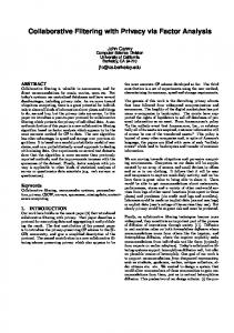
Figure 4: Performance convergence against training time on Netflix. BPR and DNS with different polynomial degrees against the real training time on Netflix. From the result we can see that within the same training time, DNS with the higher polynomial degree has a higher NDCG@5 performance, and DNS has a faster convergency, which indicates that our approach also has improvement on efficiency.
5.
CONCLUSION AND FUTURE WORK
In this paper, we have proposed the dynamic negative item sampling strategies to optimize the rank biased performance measures for top-N CF tasks. Experimental results on three well-known large-scale CF datasets verify the effectiveness and efficiency improvement of our approach. In the future work, we plan to leverage the dynamic negative item sampling approaches to optimize other measures in recommender systems such as item serendipity and freshness.
6.
REFERENCES
[1] C. Burges, R. Ragno, and Q. V. Le. Learning to rank with nonsmooth cost functions. In NIPS, 2007. [2] N. Liu and Q. Yang. Eigenrank: a ranking-oriented approach to collaborative filtering. In SIGIR, 2008. [3] Q. Lu, T. Chen, W. Zhang, D. Yang, and Y. Yu. Serendipitous personalized ranking for top-n recommendation. In WI, 2012. [4] R. Pan, Y. Zhou, B. Cao, N. N. Liu, R. Lukose, M. Scholz, and Q. Yang. One-class collaborative filtering. In ICDM, 2008. [5] S. Rendle, C. Freudenthaler, Z. Gantner, and L. Schmidt-Thieme. Bpr: Bayesian personalized ranking from implicit feedback. In UAI, 2009. [6] Y. Shi, A. Karatzoglou, L. Baltrunas, M. Larson, A. Hanjalic, and N. Oliver. Tfmap: optimizing map for top-n context-aware recommendation. In SIGIR, 2012. [7] Y. Shi, A. Karatzoglou, L. Baltrunas, M. Larson, N. Oliver, and A. Hanjalic. Climf: learning to maximize reciprocal rank with collaborative less-is-more filtering. In RecSys, 2012. [8] Y. Shi, M. Larson, and A. Hanjalic. List-wise learning to rank with matrix factorization for collaborative filtering. In RecSys, 2010. [9] M. Weimer, A. Karatzoglou, Q. Le, A. Smola, et al. Cofirank-maximum margin matrix factorization for collaborative ranking. In NIPS, 2007. [10] D. Yang, T. Chen, W. Zhang, Q. Lu, and Y. Yu. Local implicit feedback mining for music recommendation. In RecSys, 2012.