Ordinal Classification Using Hybrid Artificial Neural Networks with ...

Ordinal Classification Using Hybrid Artificial Neural Networks with Projection and Kernel Basis Functions M. Dorado-Moreno, P.A. Guti´errez, and C. Herv´as-Mart´ınez Department of Computer Science and Numerical Analysis, University of C´ ordoba, Campus de Rabanales, 14071, C´ ordoba, Spain {i92domom,pagutierrez,chervas}@uco.es http://www.uco.es/ayrna

Abstract. Many real life problems require the classification of items into naturally ordered classes. These problems are traditionally handled by conventional methods intended for the classification of nominal classes, where the order relation is ignored. This paper proposes a hybrid neural network model applied to ordinal classification using a possible combination of projection functions (product unit, PU) and kernel functions (radial basis function, RBF) in the hidden layer of a feed-forward neural network. A combination of an evolutionary and a gradient-descent algorithms is adapted to this model and applied to obtain an optimal architecture, weights and node typology of the model. This combined basis function model is compared to the corresponding pure models: PU neural network, and the RBF neural network. Combined functions using projection and kernel functions are found to be better than pure basis functions for the task of ordinal classification in several datasets. Keywords: Ordinal Classification, Projection basis functions, Kernel basis functions, Evolutionary neural networks, Evolutionary algorithm, Gradient-descent algorithm.

1

Introduction

In the real world, there are many supervised learning problems referred to as ordinal classification, where examples are labeled by an ordinal scale [24]. For instance, a teacher who rates his students using labels (A,B,C,D) that have a natural order among them (A>B>C>D). In this paper, we are selecting artificial neural networks to face this kind of problems. They are a very flexible modeling technique, whose computing power is developed using an adaptive learning process. Properties of artificial neural networks made them a common tool when successfully solving classification problems [15,17]. The objective of this paper is to adapt the hybrid model previously proposed in [14] to ordinal regression, adding a local search algorithm to result in a hybrid training method with both evolutionary and gradient-directed algorithms. E. Corchado et al. (Eds.): HAIS 2012, Part II, LNCS 7209, pp. 319–330, 2012. c Springer-Verlag Berlin Heidelberg 2012 

320

M. Dorado-Moreno, P.A. Guti´errez, and C. Herv´ as-Mart´ınez

There are a lot of models for ordinal classification [16,23], but one of the first models specifically designed for this problem, and the one our work is based on, is the Proportional Odds Model (POM). This model is based on the assumption of stochastic ordering of the input space, and the way it works is described in [26]. In this paper, the hybrid neural network proposed in [14] is combined with the POM model to face ordinal regression. Different types of neural networks are nowadays being used for classification purposes, including neural networks based on sigmoidal basis (SU), radial basis function (RBF) [21] and a class of multiplicative basis function, called product unit (PU) [25,28]. The combination of different basis functions in the hidden layer of a neural network has been proposed as an alternative to traditional neural networks [24]. We use RBF neurons and PU neurons according to Cohen and Intrator insights [8], based on the duality and complementary properties of projection-based functions (SU and PU) and kernel typology (RBF). These models has been also theoretically justified by Donoho [10], who demonstrated that any continuous function can be decomposed in two mutually exclusive functions, such as radial (RBF) and crest ones (SU and PU). In this way, RBF neurons contribute to a local recognition model [4], while PU neurons contribute to a global recognition one [25]. The combination of them results in a high degree of diversity because the submodels disagree one another. In a recent proposal [14], it is shown how the different combinations among these types of neurons can be achieved by an evolutionary algorithm. In order to adjust the neural network architecture [20] which approximates the ordinal classification problem needs, training algorithms are used. One can consider gradient-directed methods such as Back-Propagation [6], which is an algorithm based on a gradient-directed search [12] resulting in a local searching. Additionally, Evolutionary Algorithms (EAs) [5,29] are an alternative, which provide a very successful platform for optimizing network weights and architecture simultaneously. Many researchers have shown that EAs perform well for global searching, because they are capable of finding promising regions in the whole search space. In this paper we will show how a hybridization of these two types of training algorithms performs very good, first performing global search with the EA and then performing a local search in the result obtained by the EA using a gradient-directed algorithm [19]. The rest of the paper is organized as follows. Section 2 discusses how the model proposal works. In section 3, the hybrid algorithm is shown. Section 4 includes the experiments: experimental design, information about the datasets, results of the experiments and statistical analysis of the results. Finally, in section 5, we present the conclusions of the paper.

2

Model

We first propose an adaption of the classical POM model [26] to artificial neural networks. Since we are using the POM model and artificial neural networks, we can say that our proposal doesnt assure monotonicity. The way the POM model

Ordinal Classification Using HANNs with Projection and Kernel Functions

321

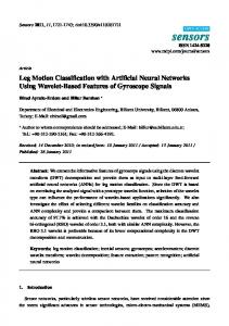
works is based on two elements: the first one is a linear layer with only one node (as seen in Fig. 1) [3], whose inputs are the non-linear transformations of a first hidden layer. The task of this node is to stamp the values into a line, to make them have an order, which allows an ordinal classification easier. After this one node linear layer, an output layer is included with one bias for each class, whose objective is to classify the patterns in the class they belong to. This classification structure corresponds to the POM model [26], which, as the majority of existing ordinal regression models, can be represented in the following general form: ⎧ c1 , if f (x, θ) ≤ β01 ⎪ ⎪ ⎪ ⎨c , if β 1 < f (x, θ) ≤ β 2 2 0 0 C(x) = , (1) ⎪ · · · ⎪ ⎪ ⎩ cJ , if f (x, θ) > β0J−1 where β01 < β02 < · · · < β0J−1 (this will be the most important constraint in order to adapt the normal classification model to ordinal classification), J is the number of classes, x is the input pattern to be classified, f (x, θ) is a ranking function and θ is the vector of parameters of the model. Indeed, the analysis of (1) uncovers the general idea previously presented: patterns, x, are projected to a real line by using the ranking function, f (x, θ), and the biases or thresholds, β0i , are separating the ordered classes. The POM model approximates f (x, θ) by a simple linear combination of the input variables, while our model considers a non-linear basis transformation of the inputs. Let us formally define the model. For each class: fl (x, θ, β0l ) = f (x, θ) − β0l ; 1 ≤ l ≤ J − 1, where the projection function f (x, θ) is estimated with the combination of a pair of basis functions: f (x, θ) = β0 +

m1 

β1,j B1,J (x, w1,j ) +

j=1

m2 

β2,j B2,j (x, w2,j ),

j=1

replacing B1,j (x, w1,j ) and B2,j (x, w2,j ) by RBFs: 

x − cj 2 B1,j (x, w1,j ) = B1,j (x, (cj , rj )) = exp − 2rj2

 ,

and PUs, respectively: B2,j (x, w2,j ) =

k i=1

w

xi 2,ji .

By using the POM model, this projection can be used to obtain the cumulative probabilities, cumulative odds and comulative logits of the ordinal regression in the following way [26]:

322

M. Dorado-Moreno, P.A. Guti´errez, and C. Herv´ as-Mart´ınez




 

 

 





   

 

   




 






 





 

  
































  


 



 















       











































 





















      

Fig. 1. Proposed hybrid model for ordinal regression

P (Y ≤ l) = P (Y = 1) + · · · + P (Y = l), P (Y ≤ l) , odds(Y ≤ l) = 1 − P (Y ≤ l)

 P (Y ≤ l) logit(Y ≤ l) = ln = f (x, θ) − β0l , 1 − P (Y ≤ l) 1 P (Y ≤ l) = ; 1 ≤ l ≤ J − 1, 1 + exp(f (x, θ) − β0l ) P (Y ≤ J) = 1, where P (Y = j) is the individual probability of a patter to belong to class j, P (Y ≤ l) is the probability of a pattern to belong to class 1 to l and the logit is modeled by using the ranking function, f (x, θ), and the corresponding bias, β0l .

Ordinal Classification Using HANNs with Projection and Kernel Functions

323

We can come back to P (Y = l) from P (Y ≤ l): P (Y = 1) = g1 (x, θ, β) = P (Y ≤ 1) P (Y = l) = gl (x, θ, β) = P (Y ≤ l) − P (Y ≤ l − 1), l = 2, . . . , J, and the final model can be expressed as: 1 , 1 + exp(f1 (x, θ, β01 )) 1 1 gl (x, θ, β) = − , l = 2, . . . , J − 1, l 1 + exp(fl (x, θ, β0 )) 1 + exp(fl−1 (x, θ, β0l−1 )) 1 gJ (x, θ, β) = 1 − . 1 + exp(fJ−1 (x, θ, β0J−1 )) g1 (x, θ, β) =

In order to hybridize the model, we use a percentage of RBF neurons and a percentage of PU neurons. Their training consists of firstly giving their weights (w1,j and w2,j ) random values to evolve them with the EA to get a global scope, and then, when they have better performance, applying the gradient-directed algorithm, to improve the model accuracy.

3

Algorithm

In this section, the hybrid algorithm to estimate the architecture and parameters of the model is presented. The objective of the algorithm is to design an hybrid neural network with optimal structure and weights for each ordinal classification problem. This algorithm is an extension of the neural net evolutionary programming proposed in a previous work [14]. In order to adapt the algorithm to ordinal classification, we have modified the codification of the individuals to fit the model given in section 2. The constraints, also mentioned in section 2, are β00 < β01 < ... < β0J−1 , J being the number of classes. The algorithm is presented in Fig. 2. To fulfill the constraints in the biases, our algorithm implements a mirror based repair of inconsistent mutation of the evolutionary part. Imagine that, after a parametric mutation, β00 > β01 so the constraints are not being fulfilled, their difference being d = β00 −β01 . Our simple proposal to repair this inconsistent mutation is to move β00 so that the distance to β01 is the same, but fulfilling the constraints, that is, β00 = β00 − 2d. The function used to evaluate the models and to get their fitness has also been adapted to ordinal regression. A weighted mean squared error (WeightedMSE) has been implemented, which is given by the following expression: l(β, θ) = −

N J

2 1  c(yn , l) ∗ gl (x, θ, β) − yn(l) , N n=1 l=1

(0)

(1)

(J)

where several symbols must be clarified: yn = (yn , yn , . . . , yn ) is a 1-of-J (j) encoding vector of the label from pattern xn (i.e. yn = 1 if the pattern xn

324

M. Dorado-Moreno, P.A. Guti´errez, and C. Herv´ as-Mart´ınez

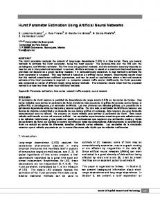
1. Generate a random population of size NP, where each individual presents a combined basis function structure 2. Repeat until the stopping criterion is fulfilled 2.1. Calculate the fitness (decreasing transformation of weighted MSE error) of every individual in the population and Rank the individuals respecto to their Weighted MSE error. 2.2. Select and store best MSE individual. 2.3. The best 10% of population individuals are replicated and substitute the worst 10% of individuals 2.4. Apply the mutations: 2.4.1. Parametric mutation to the best 10% of individuals. 2.4.2. Structural mutation to the remaining 90% of individuals using a modified add node mutation in order to preserve the combined basis function structure. 2.5. Add the best MSE individual from previous generation to the new population. 3. Select the best MSE individual in the final population. 4. Apply a gradient-directed algorithm to the best individual and consider it as a possible solution. Fig. 2. General framework of combined basis function evolutionary programming algorithm for ordinal regression

belongs to class j, and 0 otherwise), yn is the corresponding rank (i.e. yn = (j) argj (yn = 1)), β = (β01 , ..., β0J−1 ) and θ are the vector of biases and the vector of parameters of the ranking function, respectively, and c(yn , l) is a cost function in the following form:  (J/2)(J − 1), if yn = l c(yn , l) = . if yn = l |yn − l|, Let us illustrate the rationale behind this cost function with a problem of J = 4 classes. The cost of misclassifiations will be organized with the following cost matrix: ⎛ ⎞ 6123 ⎜1 6 1 2⎟ ⎟ C4 = ⎜ ⎝2 1 6 1⎠, 3216 in such a way that the errors between individual predicted probabilities and actual ones of the M SE are differently penalized depending how far the class analyzed is from the correct class. If the class is incorrect, the penalization is the absolute value of the difference in rank. If the class is correct, the penalization is as high as the sum of the penalizations for the incorrect ones (which is J/(2(J − 1)), i.e. the sum of the natural numbers from 1 to J − 1). The final step is to apply the gradient-search algorithm, which is iRP rop+ [18]. For using this algorithm, we obtained the derivatives for the model of section 2, taking into account that we have two different types of basis functions.

Ordinal Classification Using HANNs with Projection and Kernel Functions

4

325

Experiments

In order to analyze the performance of the hybrid basis function model and the corresponding hybrid training algorithm, six datasets have been tested, their characteristics shown in Table 1. The collection of datasets is taken from the UCI [1] and the mldata.org [27] repositories. Table 1. Characteristics of the six datasets used for the experiments: number of instances (Size), inputs (#In.), classes (#Out.) and patterns per-class (#PPC) Dataset Size #In. #Out. #PPC car 1728 21 4 (1210,384,69,65) ESL 488 4 9 (2,12,38,100,116,135,62,19,4) LEV 1000 4 5 (93,280,403,197,27) SWD 1000 10 4 (32,352,399,217) tae 151 54 3 (49,50,52) toy 300 2 5 (35,87,79,68,31)

The following two measures have been used for comparing the models: 1. CCR: The Correct Classification Rate (CCR) is the rate of correctly classified patterns: N 1 ∗ CCR = y = yi , n i=1 i where yi is the true label, yi∗ is the predicted label and · is a Boolean test which is 1 if the inner condition is true. CCR values range from 0 to 1. It represents a global performance on the classification task. This measure is not taking into account category order. 2. M AE: The Mean Absolute Error (M AE) is the average deviation in absolute value of the predicted class from the true class [2]: N

M AE =

1 e(xi ), n i=1

where e(xi ) = |yi − yi∗ | is the distance between the true and the predicted ranks, and M AE values range from 0 to J − 1. This a way of evaluating the ordering performance of the classifier. 3. Kw : The weighted Kappa is a modified version of the Kappa statistic calculated to allow assigning different weights to different levels of aggregation between two variables [11]: Kw = where

po(w) − pe(w) , 1 − pe(w) J

po(w) =

J

1  wij nij , n i=1 j=1

326

M. Dorado-Moreno, P.A. Guti´errez, and C. Herv´ as-Mart´ınez

and pe(w)

J J 1  = 2 wij ni· n·j , n i=1 j=1

where nij represents the number of times the patterns are predicted by the J classifier to be in class j when they really belong to class i, ni· = j=1 nij J and n·j = i=1 nij for i, j = 1, ..., J. The weight wij quantifies the degree of discrepancy between the true (yi ) and the predicted (yj∗ ) categories, and Kw values range from −1 to 1. All the parameters of the algorithm are common to these six problems. The main parameters of the algorithm are: minimum and maximum number of hidden nodes (m = 10 and M = 25, respectively), population size (NP = 500), number of generations (GE = 350), number of iterations in the local search (GLS = 500) and percentage of the different types of hidden neurons (pRBF = 15% and pPU = 85%). Note that the algorithm is run exactly with the same model, parameters and conditions both for pure and hybrid neural network models. An analysis of the results obtained for both RBF and PU pure models compared with the hybrid model is performed for every dataset. We have also included two state-of-the-art classifiers: – GPOR: Gaussian Processes for Ordinal Regression. GPOR [7] is a Bayesian learning algorithm, where the latent variable f (x) is modelled using Gaussian Processes, and then all the parameters are estimated by using a Bayesian framework. The authors of GPOR provide publicly available software implementations of the methods1 . For GPOR-ARD no hyper-parameters were set up since the method optimizes the associated parameters itself. – EBC-SVM: this method applies the Extended Binary Classification (EBC) procedure to SVM [22]. The EBC method can be summarized in the following three steps. First, transform all training samples into extended samples weighting these samples by using the absolute cost matrix. Second, all the extended examples are jointly learned by a binary classifier with confidence outputs, aiming at a low weighted 0/1 loss. Last step is used to convert the binary outputs to a rank. In this way, EBC is a specific method for ordinal regression based on reformulating the problem as a binary classification problem. The hyperparameters were adjusted using a nested 10-fold cross-validation over the training set with the following values: width of the kernel,γ ∈ {10−3, 10−2 , ..., 103 }, and cost parameter, C ∈ {10−3 , 10−2 , ..., 103 }. The evaluation measure was the test M AE error. Both methods were configured for using the Gaussian kernel. For the neural network methods, the experimental design was conducted using 10 random holdout procedures with 3 repetitions per holdout, 3n/4 instances for the training set and n/4 instances for the generalization set (where n is the size of the dataset). For the EBC(SVM) and GPOR methods, a total of 30 random holdout procedures are performed, because of their deterministic nature. 1

GPOR (http://www.gatsby.ucl.ac.uk/~ chuwei/ordinalregression.html)

Ordinal Classification Using HANNs with Projection and Kernel Functions

327

Table 2. Results of the different methods evaluated, considering test CCR, M AE and Kw CCR(%) M AE Func. Mean ± SD Mean ± SD Hybrid 97.5231 ± 1.0927 0.0251 ± 0.0112 PU 97.3688 ± 1.2758 0.0267 ± 0.0132 RBF 97.0756 ± 1.6497 0.0305 ± 0.0170 GPOR 96.2814 ± 0.9334 0.0376 ± 0.0098 EBC(SVM) 97.7392 ± 0.8438 0.0226 ± 0.0084 ESL Hybrid 72.7595 ± 2.5891 0.2887 ± 0.0253 PU 72.1584 ± 4.1599 0.2942 ± 0.0388 RBF 70.9016 ± 2.7796 0.3035 ± 0.0271 GPOR 71.3115 ± 3.0669 0.3008 ± 0.0346 EBC(SVM) 71.1749 ± 3.4177 0.3046 ± 0.0381 LEV Hybrid 62.4266 ± 3.1756 0.4032 ± 0.0343 PU 61.1733 ± 3.5606 0.4176 ± 0.0413 RBF 62.4000 ± 3.0876 0.4034 ± 0.0331 GPOR 61.2267 ± 3.0116 0.4219 ± 0.0308 EBC(SVM) 62.3600 ± 2.3477 0.4133 ± 0.0264 SWD Hybrid 57.2133 ± 3.2419 0.4376 ± 0.0388 PU 57.0800 ± 3.2583 0.4498 ± 0.0401 RBF 55.6667 ± 2.6967 0.4724 ± 0.0302 GPOR 57.3377 ± 3.0548 0.4401 ± 0.0323 EBC(SVM) 56.6800 ± 3.1111 0.4502 ± 0.0323 tae Hybrid 61.4912 ± 5.6349 0.5035 ± 0.0723 PU 60.7894 ± 5.4130 0.5131 ± 0.0617 RBF 54.1052 ± 7.3863 0.5526 ± 0.0854 GPOR 32.8070 ± 4.0729 0.8614 ± 0.1551 EBC(SVM) 52.1930 ± 7.3491 0.5149 ± 0.0865 toy Hybrid 96.6667 ± 1.6329 0.0333 ± 0.0163 PU 75.3333 ± 8.6321 0.2640 ± 0.1071 RBF 94.0000 ± 3.1659 0.0600 ± 0.0316 GPOR 95.3370 ± 2.2340 0.0462 ± 0.0223 EBC(SVM) 96.5778 ± 2.4928 0.0342 ± 0.0212 The best result is in bold face and the second one in italics Dataset car

Kw Mean ± SD 0.9884 ± 0.0065 0.9431 ± 0.0267 0.9367 ± 0.0348 0.9396 ± 0.0162 0.9639 ± 0.0132 0.6930 ± 0.0142 0.6505 ± 0.0514 0.6340 ± 0.0346 0.8010 ± 0.0227 0.7982 ± 0.0264 0.5172 ± 0.0145 0.4445 ± 0.0513 0.4608 ± 0.0468 0.5459 ± 0.0374 0.5700 ± 0.0326 0.4361 ± 0.0183 0.3418 ± 0.0492 0.3210 ± 0.0465 0.4390 ± 0.0427 0.4310 ± 0.0423 0.4223 ± 0.0842 0.4117 ± 0.0808 0.3565 ± 0.1106 0.3693 ± 0.2268 0.3378 ± 0.1102 0.9666 ± 0.0211 0.6758 ± 0.1146 0.9217 ± 0.0414 0.9642 ± 0.0175 0.9737 ± 0.0175

Table 2 shows the mean test value and standard deviation of the correct classified rate (CCR) and the mean absolute error (M AE) over the 30 models obtained (10 holdout procedures ×3 repetitions or 30 holdout procedures). If we take into account the accuracy measure, the hybrid model with PUs and RBFs outperforms all the other models for 4 out of the 6 datasets. The number of datasets where the hybrid models obtain the best M AE results is 5 datasets, achieving the second best performance for the remaining one. Although the results seem to present the hybrid model as the best performing one, it is necessary to ascertain the statistical significance of the differences observed. We follow the guidelines of Demsar [9] to achieve this purpose.

328

M. Dorado-Moreno, P.A. Guti´errez, and C. Herv´ as-Mart´ınez

Table 3. Average rankings (R) of the different methods evaluated, considering test CCR, M AE and Kw CCR M AE Kw Method R p-value R p-value R p-value α(0.1,Holm) Hybrid 1.33 − 1.25 − 2.00 − − 3.25 0.005• 3.83 0.008• 0.025 PU 3.33 0.006• 3.75 0.006• 4.42 0.045 0.033 RBF 3.83 0.018• 3.83 0.028• 2.42 0.648 0.050 GPOR 3.50 0.028• 0.100 EBC(SVM) 3 .00 0.068• 2 .92 0.068• 2 .33 0.715 The best result is in bold face and the second one in italics •: statistically significant differences for α = 10%

A non-parametric Friedman test [13] has been carried out with the CCR and M AE rankings of the different methods (since a previous evaluation of the C and M AE values results in rejecting the normality and the equality of variances hypothesis). The ranking is obtained for each dataset and each measure in the following way: R = 1 is assigned to the best method for this measures and dataset, and R = 5 is assigned to the worst one. The average value of this rankings are included in Table 3. The Friedman test shows that the effect of the method used for classification is statistically significant, as the confidence intervals are C0.1 = (0, F0.1 = 2.25) and C0.05 = (0, F0.05 = 2.87) and the Fdistribution statistical values are F ∗ = 3.11 ∈ / C0.05 for C, F ∗ = 3.91 ∈ / C0.05 for ∗ / C0.05 for Kw . Consequently, the null-hypothesis stating M AE and F = 4.07 ∈ that all algorithms perform equally in mean ranking is rejected for all measures. Based on this rejection, the Holm post-hoc test is used to compare all classifiers to each other. Holm test is a multiple comparison procedure that considers a control algorithm and compares it with the remaining methods [9]. Holm’s test adjusts the value for α in order to compensate for multiple comparison. The test is a step-up procedure that sequentially checks the hypotheses ordered by their significance. The results of the Holm test for α = 0.10 can also be seen in Table 3, using the corresponding p and α(0.1,Holm) values. From the results of this test, it can be concluded that the Hybrid methodology obtains a significantly higher ranking of CCR and M AE when compared to all the remaining methods, which justifies the proposal. The ranking of Kw is significantly higher than that of P U method.

5

Conclusions

A new neural network model has been proposed to face ordinal regression problems, which is mainly based on projecting the patterns into a real line and interpreting the output of the net using the Proportional Odds Model (POM) framework with a different threshold for each class, to transform them in ordered probabilities. A previously proposed nominal hybrid model, based on combining different basis functions, has been adapted to this framework, adjusting the corresponding evolutionary algorithm and including a final local search step.

Ordinal Classification Using HANNs with Projection and Kernel Functions

329

The new hybrid ordinal regression neural network has been compared to the corresponding pure models which is composed of (Product Unit neural network, PU, Radial Basis Function neural network, RBF) for a total of 6 datasets, including statistical tests to evaluate the significance of the result differences. Additionally, Extended Binary Classification for Support Vector Machines [EBC(SVM)] and Gaussian Processes for Ordinal Regression (GPOR) have also been considered. Our findings reveal that, for this set of datasets, the hybrid model proposed is significantly better than the pure models and EBC(SVM) and GPOR for two of the three measures considered (accuracy and mean absolute error) and it is better (although without statistically significant differences) for the Kw measure. Acknowledgments. This work has been partially subsidized by the TIN201122794 project of the Spanish Inter-Ministerial Commission of Science and Technology (MICYT), FEDER funds and the P08-TIC-3745 project of the “Junta de Andaluc´ıa” (Spain).

References 1. Asuncion, A., Newman, D.: UCI machine learning repository (2007), http://www.ics.uci.edu/~ mlearn/MLRepository.html 2. Baccianella, S., Esuli, A., Sebastiani, F.: Evaluation measures for ordinal regression. In: Proceedings of the Ninth International Conference on Intelligent Systems Design and Applications (ISDA 2009), Pisa, Italy (December 2009) 3. Bishop, C.M.: Pattern Recognition and Machine Learning. Information Science and Statistics, 1st edn. Springer, Heidelberg (2006) 4. Bishop, C.: Improving the generalization properties of radial basis function neural networks. Neural Computation 8, 579–581 (1991) 5. Castro, L.N., Hruschka, E.R., Campello, R.J.G.B.: An evolutionary clustering technique with local search to design rbf neural network classifiers. In: Proceedings of the IEEE International Joint Conference on Neural Networks, pp. 2083–2088 (2004) 6. Chauvin, Y., Rumelhart, D.E.: Backpropagation: Theory, Architectures, and Applications. Lawrence Erlbaum Associates, Inc., Mahwah (1995) 7. Chu, W., Ghahramani, Z.: Gaussian processes for ordinal regression. Journal of Machine Learning Research 6, 1019–1041 (2005) 8. Cohen, S., Intrator, N.: A hybrid projection-based and radial basis function architecture: initial values and global optimisation. Pattern Analysis & Applications 5, 113–120 (2002) 9. Demˇsar, J.: Statistical comparisons of classifiers over multiple data sets. Journal of Machine Learning Research 7, 1–30 (2006) 10. Donoho, D.: Projection-based approximation and a duality with kernel methods. The Annals of Statistics 5, 58–106 (1989) 11. Fleiss, J.L., Cohen, J., Everitt, B.S.: Large sample standard errors of kappa and weighted kappa. Psychological Bulletin 72(5), 323–327 (1969) 12. Fletcher, R., Reeves, C.M.: Function minimization by conjugate gradients. Computer Journal 7, 149–154 (1964) 13. Friedman, M.: A comparison of alternative tests of significance for the problem of m rankings. Annals of Mathematical Statistics 11(1), 86–92 (1940)

330

M. Dorado-Moreno, P.A. Guti´errez, and C. Herv´ as-Mart´ınez

14. Guti´errez, P.A., Herv´ as-Mart´ınez, C., Carbonero-Ruz, M., Fernandez, J.C.: Combined projection and kernel basis functions for classification in evolutionary neural networks. Neurocomputing 27(13-15), 2731–2742 (2009) 15. Guti´errez, P.A., Lopez-Granados, F., Pe˜ na-Barrag´ an, J.M., Jurado-Exp´ osito, M., G´ omez-Casero, M.T., Herv´ as-Mart´ınez, C.: Mapping sunflower yield as affected by Ridolfia segetum patches and elevation by applying evolutionary product unit neural networks to remote sensed data. Computers and Electronics in Agriculture 60(2), 122–132 (2008) 16. Hecht-Nielsen, R.: Neurocomputing. Addison-Wesley (1990) 17. Herv´ as-Mart´ınez, C., Garcia-Gimeno, R.M., Mart´ınez-Estudillo, A.C., Mart´ınezEstudillo, F.J., Zurera-Cosano, G.: Improving microbial growth prediction by product unit neural networks. Journal of Food Science 71(2), M31–M38 (2006) 18. Igel, C., H¨ usken, M.: Empirical evaluation of the improved rprop learning algorithms. Neurocomputing 50(6), 105–123 (2003) 19. Ishibuchi, H., Yoshida, T., Murata, T.: Balance between genetic search and local search in hybrid evolutionary multi-criterion optimization algorithms. IEEE Transactions on Evolutionary Computation 7(2), 204–223 (2003) 20. Koza, J.R., Rice, J.P.: Genetic generation of both the weights and architecture for a neural network. In: Proceedings of International Joint Conference on Neural Networks, vol. 2, pp. 397–404. IEEE Press, Seattle (1991) 21. Lee, S.H., Hou, C.L.: An art-based construction of RBF networks. IEEE Transactions on Neural Networks 13(6), 1308–1321 (2002) 22. Li, L., Lin, H.T.: Ordinal Regression by Extended Binary Classification. In: Advances in Neural Information Processing Systems, vol. 19, pp. 865–872 (2007) 23. Lievens, S., Baets, B.D.: Supervised ranking in the weka environment. Information Sciences 180(24), 4763–4771 (2010), http://www.sciencedirect.com/science/article/pii/S0020025510002756 24. Lippmann, R.P.: Pattern classification using neural networks. IEEE Transactions on Neural Networks 27, 47–64 (1989) 25. Mart´ınez-Estudillo, A.C., Mart´ınez-Estudillo, F.J., Herv´ as-Mart´ınez, C., Garc´ıa, N.: Evolutionary product unit based neural networks for regression. Neural Networks 19(4), 477–486 (2006) 26. McCullagh, P.: Regression models for ordinal data (with discussion). Journal of the Royal Statistical Society 42(2), 109–142 (1980) 27. PASCAL: Pascal (pattern analysis, statistical modelling and computational learning) machine learning benchmarks repository (2011), http://mldata.org/ 28. Schmitt, M.: On the complexity of computing and learning with multiplicative neural networks. Neural Computation 14, 241–301 (2001) 29. Yao, X.: Evolving artificial neural networks. Proceedings of the IEEE 87(9) (1999)