packed of chicken pieces. ..... Pieces suffer a cleaning process during the stay in the ... Period. Period piece cleaner image copy number of pieces detection.
Organised neural networks and its use in real-time environments * G. Andreu, A. Crespo and J. Simó Departamento de Ingeniería de Sistemas, Computadores y Automática Universidad Politécnica de Valencia {gandreu,alfons,jsimo}@disca.upv.es
Abstract.
is implemented in a monoprocessor system and it has to operate under real time constraints.
? Self-organising feature maps (SOFM) are an important tool to visualize high-dimensional data as a twodimensional image. One of the possible application of this network is to image recognition. However, this architecture presents some problems mainly due to the border effects. In this paper a new organisation of feature maps named toroidal self-organising feature maps (TSOFM) is presented. Its main advantage is the elimination of the border effects and, consequently, the increasing of the rate of the recognition. Another important aspect presented in this paper is the measurement of how well organised is the networks during the training phase. This proposal have been experimented in an industrial application demonstrating the better quality results.
In this paper two original improvements of this kind of networks will be presented. A first proposal related to the network structure, the network is organised as a toroidal topology avoiding the border effects. As result of this topology all nodes have the same number of neighbours and an uniformity for node computation is obtained. The second one is associated to the operation in real time environments of the network: a measurement of the organisation degree of a network: it permits to generate several neural networks with different number of nodes that can be used, depending on the available time, to obtain the best answer with the available time.
Keywords: Neural networks, vision systems, real-time measurement and control
Introduction. The self-organising feature map (SOFM) were originally proposed by Kohonen [Koh 84] as a way of representing high-dimensional data in a twodimensional space to facilitate visual inspection data. Several applications can be found in the literature about the SOFM as image compression [Karen 95], recognition activities [Andreu 90]. Several modifications have been proposed to reduce the training and the formation map costs. One of the problems that appears in these networks is due to the asymmetry of the architecture. The nodes located in the extreme of the network belong to less number of neighbourhoods that the internal nodes. This fact, that was observed in the traditional learning method [Koh 81], [Rodrigues 91], produces a distortion in the nodes near the border. This phenomenon, known as the border effects, requires to be reduced to achieve better recognition results. Several works [Rodrigues-91], [Truong-91] propose some criteria to reduces these effects. It reduces the recognition level of the network. A more general problem is presented when the network ?
* This work has been funded by grant No. TAP-0511C02 of the Spanish Government
The proposal has been applied to the recognition and packed of chicken pieces.
Definitions. A TSOFM is denoted by ? ?= {N, ?, p} , where N is the set of nodes, ??the weight vector, and p an application p: N? ?? that establish the correspondence of each node of the N set and one weight vector in the ??set. In the architecture of a TSOFM, nodes in the first row are neighbours of nodes in the last row. In the same way, nodes located in the first column and the last column are neighbours. As consequence, the four nodes located in the corners are neighbours. The major difference between the SOFM and TSOFM is that all nodes have the same number of topological neighbourhoods in all directions. The topological distance D(n i,j, n l,k) between two nodes n i,j, nl,k ? N in the network ? ?= {N, ?, p} can be defined as:
D(ni,j, nl,k) = |i-l| + |j-k| where |i-l| represents the row topological distance and |j-k| the column topological distance between these nodes. The topological neighbourhood ? ri,j= {N ri,j , ? ri,j, p} is r defined as a sub-network of ? , ? i,j ? ? , where r represent the topological ratio, N ri,j= {n l,k : max(1,i-r)?
l ? min(f,i+r), max(k,j-r)? k ? min(c,j+r)} and ? ri,j= {? l,k : max(1,i-r)? l ? min(f,i+r), max(k,j-r)? k ? min(c,j+r)}. The SOFM traditional algorithm [Lippman 87] can be described as follows: In the first step, the weight vectors set ? are initialised to random values. Each iteration in the learning process consists on three sequential steps: i) the presentation of a randomly chosen input vector from the input space, ii) the selection the n i,j with smallest Euclidean distance at the input vector, and iii) the updating of the weight vectors included in ? ri,j. In the following, the iteration will be indexed by time ?? and, the weight vectors are updated according to the next procedure:
?
?? ? ( t ? 1 ) ? ? l, k ?? ?
l, k
l, k
?
( t ) ? ? ( t ) x( t ) ?
?
l, k
(t )
?
(t )
if
n
if
l, k
n
?
l, k
?
?
?
r i ,j
There are different studies in the literature about how the SOFM preserve the input data topology [Martin 95], [Kangas 90]. But there are no references how many times should be trained with the input data to obtain the best SOFM organisation. An important aspect that can help to decide if it is necessary to give more times the data set to the network is to quantify how well organised is a network during the learning phase. If the network is well organised new input data do not increment the organisation and, as consequence, it is unnecessary. This section introduces a new parameter called organisation degree. This parameter quantifies the optimum number required to give the data set to the TSOFM to obtain the best organised network. A network ? = {N, ?, p} is well organised if ? n i,j, nl,k, n p,q ? N, with DT(n i,j, n l,k)=1, DT(n i,j, n p,q)>1, then
where
?
?
l ,k
?
?
i, j
?
?
Q D ?far ,8 _ neig ? ? ? ? D ?n ,8 _ ? G ?? ? ? Q D ?far ,8 _ neig ? ? Q D ?N ? 2
T
org
T
Q
Q
l?1
k ?1
T
2
2
T
T
l .k
l, k
?
1 T l, k
where DT(far,8_neig)=8*Q-10 is the sum of the topological distance to the eight nodes topological further a node n l,k in N; DT(n l,k,8_? l,k) is the sum of the topological distances at the eight nodes of N satisfying the Euclidean distance between weight vector of them and the weight vector of n l,k are minimum, and
r
Organisation Degree.
i, j
The organisation degree of a network ? = {N, ?, p} with an even number of rows and columns Q is defined as:
i ,j
The r integer value decreases with time t , obtaining a r ? i,j as a function of time t and shrinks monotonically. The parameter a(t) is the step size of the adaptation of the weights and also shrinks monotonically with time.
?
and useful to define an expression evaluating how much organised is a network.
p,q
represents the Euclidean distance.
A bad organised or disorganised network has no nodes that satisfy the previous equation. The previous definitions imply that all nodes of a network are well or bad organised. Usually, a network will not be completely organised or disorganised. It means we can found in a network well organised nodes and disorganised. For that reason, it is more reasonable
D (N T
1 T l ,k
) ?
l ?1
k? 1
? ? D (n , n
m? l ? 1 q ? k? 1
T
l ,k
m ,q
) ? 12
is the sum of the topological distances of the eight 1 nodes included in the N l,k .
Interiority level in labelling. The computational cost in the recognition phase is particularly very important in real time applications. In general networks with an higher number of nodes produce better results than network with less nodes. However, all the nodes in a network have not the same importance to recognition purposes. In other words, there are nodes in a network that are essential to have high rate recognition and others that are used to recognise or to identify a little part of the data. Of course all nodes are important when the best result are wanted, but in many cases, it is necessary to find an agreement between the rate recognition and the answer cost time. As result of the training process in a ? T, the nodes ? n i,j ? NT should be located in the network near to the nodes having weight vectors very similar to ? i,j. After the training process the nodes with the same label are located and clustered. A labelled network ? T*={N T*, ?T , p} can be seen as a set of labelled maps {Lx }. In NT* the nodes are identified with n i,j(t x) being tx the label. Let {C x} the set class contained in the dataset used to train the network. A class tx ? {C x} with mx nodes labelled with tx are “well mapped”, if this class have all the mx nodes located in ? T* in a way that each one of theirs have between its 8 nearest neighbour the larger number possible of the nodes labelled with the same label tx. The interiority of a node ni,j(t x) in label tx is defined as:
?N t t I ?n ?t ?? ? ? ? n ?t ? ? ? N t ? n
i,j
?
?
n
l ,k
?tn ? ?
?
n
i,j
?tx ? ?
this value has reach a good level and to stop the training process.
1 T i, j
?
n
i,j
?t x ? ?
Node elimination.
x
x
?
T i,j
1
l,k
n
n
where the numerator obtains the number of nodes in N1 Ti,j with the same label of n i,j(t x) with the exception of the ni,j(t x) and the denominator computes the number of nodes in N1 Ti,j with the exception of the n i,j(t x). Taking into account this information, it is possible to associate to a network the following information: a) global organisation degree; b) Interiority level of each label c) Required computation time This information can be used during the learning phase to determine two important aspects: 1. If the network is organised enough 2. Which nodes are more important than others in the recognition task The following figure (Figure 1) shows the evolution of the organisation degree parameter during the learning phase of three different sizes of TSOFM.
Figure 1: Organisation degree evolution of three TSOFM As it can be seen, the evolution of the organisation degree during the first iterations does not change too much. It is due to the initial random values assigned. After that, the organisation degree trends asymptotically to a value. The relation between the number of iteration with radius constant and variable detrmines the instant the organisation degree increases asymptotically. So, it is possible to determine when
The second objective is the detection of less important nodes and the evaluation of the reduction of the recognition rate. The node elimination allows to obtain less reduced networks and, as consequence, the computation time required to recognise an object. It is solved in this way because of the results obtained with large networks with node elimination are frequently better than medium or small network without it. So, the procedure is to train large, medium and small networks, to eliminate the less important nodes and to estimate the effects of the reduced networks with respect to the recognition rate. This node elimination allows an additional aspect with respect to the exposed above: 3. The expected quality of the resultant network and computation time required for a sequential implementation. Next figure 2 shows the evolution of the quality of the response (recognition rate in percentage) when less significant nodes are removed in the three TSOFM showed in figure 1.
Figure 2: Evolution of the recognition rate In each representation we show the evolution of the quality of the response of several networks (8x8, 16x16, 32x32 nodes) when nodes less significant are eliminated. It can be seen, the global quality of the response increases when some nodes are removed due to these nodes affect to the interaction between labels. It produces that a label will have decreased its quality meanwhile the global will be higher.
In the figure 2, it can be detected which are the best options for each network. Both figures have been obtained with objects like showed in figure 3 of the application.
system can easily do the required actions to analyse and classify all the objects. But if the system works in a stressed situation and the number of objects is very high, the options to handle the objects can be:
The result of this phase can be organised in a table (Table 1) with the following information:
• To analyse and classify as many objects as the system can with the same level of quality • To reduce the speed of the conveyor belt obtain more time to do all the actions • To use different actions which require less time, analyse of all them, improve the more critical.
NI
1 2 3 4 5 6 7 8 9 10 11
Network
32x32 32x32 32x32 32x32 16x16 16x16 16x16 16x16 8x8 8x8 8x8
Nodes
GRR %
NLHRR
1024 513 252 5 256 232 43 5 64 19 5
74,87 78,97 68,72 53,33 74,67 76,41 73,85 69,23 68,72 72,82 59,43
2 3 2 4 2 2 2 2 3 2 2
Table 1. Result obtained when nodes are removed. where NI is the network identifier, GRR is the global recognition rate, NLHRR is the number of labels with a recognition rate higher than the global. The expected computation time ECT of a network it is lineal with the node number. So, the node number of a network gives an idea of the computation requirement, The table shows the more representative configuration obtained after being trained several networks with the same set of data. En each network we wrote the largest network (1024, 256, and 64), the best from recognition rate point of view (513, 232, and 19), and the minimum (5 nodes) in order to compare the results. Each configuration has its own values par label. Next table (Table 2) shows the label values in two cases. Net 32x32 16x16
Nod. L1 L2 L3 L4 L5 Total 1024 95,8 73,9 69,2 56,2 69,5 74,8 232 93,7 78,2 61,5 59,3 73,2 76,4 Table 2. Detailed recognition rate for label
With this table, it is possible to build several versions of the network that can be used depending on the available time to obtain the response with more or less quality. Real time applications are software programs where actions should be taken with some temporal constraints: periods, deadlines, etc. To achieve the temporal constraints it is necessary to know in advance the activities and the worst case execution time to produce the actions. In some applications the system can work in different conditions: more or less stressed. It means that more or less actions have to be taken in the same interval. A typical application is the recognition of objects in a conveyor belt to classify them: tiles, oranges, eggs, meat pieces, etc. If the quantity of objects in the area in analysis is low the
In the application we describe, the third approach has been followed. Several networks with different expected execution time can be used to recognise objects. So, the system taking into account the number of object to be recognised will used the best option: the network with the best recognition time to the available time. If at the end of the process there is remaining time some of the objects with low recognition rate labels can be analysed again. The use of these approach is described in the next section on the basis of an application.
Application. To be able to use this approach in a real-time environment it is needed a scheduling policy able to manage activity versions. A model task to include optional tasks in a real-time environment is derived of imprecise computation model [García95]. In this work a scheduler allows the execution of a mandatory part and optional parts if there is available time to execute them. The available time is known in advance so, the scheduler can select the best network taking into account the parameters: quality of the response, and computation time. The application consists on the recognition and storagement of chicken pieces. Chickens are cut by humans and are left in a conveyor belt. A camera takes scenes that are analysed to recognise parts of chicken and to store and label in the appropriated way. A robot arm takes pieces and store them in a box. There are five classes of pieces (parts of the chicken: wing, thigh, leg, quarter, and breast). Initially, several images of the chicken parts are recorded and used to train the networks. Networks are tra ined with objects in several orientations. Figure 3 shows the different kind of pieces and orientations used to train the network.
in the limit of the work area are analysed in the current picture or the next one depending on the relation of areas inside the work and picture zones. A first analysis of the image has the objective of detecting the number of pieces and the location. The image of each piece has to be extracted of the total image and analysed. The analysis consists in the recognition of which kind of piece is and the orientation. To obtain that the image is given to the network which according to the training set answers with the recognised label. Pieces suffer a cleaning process during the stay in the conveyor belt to be finally packed.
Figure 3. Pieces of a chicken Figure 4 shows the layout of the application components. Parts of chickens are thrown to the conveyor belt. A ceiling camera takes pictures of the conveyor belt each period of time. This period is calculated taking into account the speed of the conveyor belt and the effective work area of the picture. Each period, the camera takes a picture and store it in the memory of the computer system. Pieces
Recognised pieces are stored in a data structure and picked up by the manipulator at the end of conveyor belt to store in the appropriated box. The system knows at each moment the exact position of each piece in the conveyor belt (from the acquired image affected by the time difference between it was taken and the current time) to control the robot arm to a specific position.
Camera picture area work area
Period
piece cleaner
Conveyor belt delayed time
work area
Robot arm Period image copy number of pieces detection piece recognition manipulator actuation
Figure 4. Application layout At the bottom of the figure 4 it can be seen the execution of activities related to the recognition and storagement. There is a periodic activity (period P, and global deadline D), which performs the image copy to memory, the analysis of how many objects or pieces
are in the working area, the recognition of all the pieces and the orders to the robot to get pieces and store them. These four activities are part of a task that is executed concurrently with other activities like the
control of the components in the cleaner box, the speed of the conveyor belt, and other minor tasks. The problem stated in this paper is related to the recognition activity of the pieces. Of course the number of pieces in a working area is very variable, but the most constrained part of the system from the real time operation is the robot arm. It can handle a limited number of pieces par time unit. Working at the maximum speed the recognition process can not recognise at the maximum level detail all the pieces. So, it is needed, as we commented above, that the conveyor belt reduces the speed or to use less time to analyse individually each piece. In the previous training phase, a set of networks have been identified and structured. Each network is version of the same network with different level of recognition (quality of the response), labels with less level of recognition (less organisation level), and computation time (depending on the node number of the network). From the computation time of all the tasks in the system the Deadline Monotonic Theory [Audsley95] can be use to assign priorities to these tasks and to calculate the available time [García95]. From this information, we can determine the maximum time that can be invested each period in the recognition phase without lost of the temporal constraint in the other tasks. Given this time Tm the problem is stated as how to recognise at the maximum level of quality all the n pieces in the working area. To do that, the algorithm selects the more appropriated version of the networks assuming that Tm/n is the maximum time that can be invested in each piece. The selected version will have a expected computation time ECT < Tm/n and, as consequence a small quantity of time [(ECT-Tm/n)*n] can be invested in those pieces which resultant label has an organisation level lower than the recognition rate of the network. With this approach is it possible to work, with a high level of quality in the answer , at the maximum production integrating artificial intelligence techniques in real time environments.
Conclusions. In this paper a new self-organising feature map with toroidal architecture has been presented (TSOFM). The main aspect solved in the new structure is the border effects in the learning phase which decreases the recognition rate of the traditional networks. Moreover, two original improvements of this kind of networks have been presented. The network is organised as a toroidal topology avoiding the border effects and a measurement of the organisation degree of a network: it permits to generate several neural networks with different number of nodes that can be used, depending on the available time, to obtain the best answer with the available time. The proposal has been applied to the recognition and packed of chicken pieces showing this advantages.
References
[Andreu 90] G. Andreu, E. Vidal and E. Casacuberta "An Empirical of Feature Maps and Other Clustering Thecniques for Frame Labelling of Speech", EUSIPCO-90, Sep. 1990, Barcelona. [Rodrigues 91] J. S. Rodrigues and L. B. Almeida "Improving the Learning Speed in Topological Maps of Patterns", Neural Networks: Advances and Applications, Elsevier Science Publishers B.V. (North Holland) 1991, pp. 65-78. [Truong 90] Khoan K. Truong and Russell M. Mersereau, "Structural Image Codebooks And The Self-Organizing Feature Map Algorithm", IEEE ICASPP, vol.4, pp. 22892292, April 1990. [Jain 89] R. K. Jain, “Image analysis and computer vision”. Prentice-Hall, 1989. [Karen 95] Karen L. and Robert M. Gray, “Combining Image Compression and Classification Using Vector Quantization”, IEEE Trans. on Pattern Analysis and Machine Intelligence”, vol. 17 No. 5, pp.461-473, May 1995. [Koh 81] T. Kohonen, "Analisys Of A Simple SelfOrganizing Process", Helsinki University of Technology, Report TKK-F-A462, 1981. [Koh 84] T. Kohonen. "Self-Organization and Associative Memory", Spring-Verlag Berlin Heidelberg New York 1984. [Lippman 87] R. P. Lippmam , " An Introduction To Computing With Neural Nets", IEEE ASSP Magazine, pp. 4-21, April 1987. [Martin 95] Martin A. Kraaijveld, Jianchang Mao and Anil K. Jain “A Nonlinear Projection Method Based on Kohonen´s Topology Preserving Maps” in IEEE Transactions on Neural Networks, vol. 6 NO. 3, pp. 548-559, May 1995. [Kangas 90] Kangas J. A., Kohonen T. K. and Laaksonen J.T. “Variants of Self-Organizing Maps”, in IEEE Trans. Neural Networks, Vol. 1, NO. 1, pp. 93-99, March 1990. [Truong 91]Khoanh K.Truong "Multilayer Kohonen Image Codebooks With a Logarithmic Search Complexity", IEEE ICASSP May 1991. [Audsley 95] Audsley, N.C., Burns, A., Davis, R., Tindell, K., and Wellings,J. (1995). "Fixed priority pre-emptive scheduling: an historical perspective". Real-Time Systems 8, 173-198 (1995). [García 95] Garcia-Fornes A., Crespo, A., and Botti, V. (1995). "Adding hard real-time tasks to artificial intelligence environments". 20th WRTP, Fort Lauderdale,Florida, USA.