underlying network can be represented as a graph G V; E where the set of ... time and d v is the deadline time; these are the earliest and ... network lie on a line i.e., if nodes can be ordered as v1; v2;:::;vn .... with every pair u; v of vertices; Tu;v is the cost of an opti- .... (respectively C i; j;R ) be the cost of uniform route on net-.
Parallel Algorithms for Vehicle Routing Problems K. Jeevan Madhu� Sanjeev Saxena Computer Science & Engineering, Indian Institute of Technology, Kanpur, INDIA-208 016
Abstract In a complete directed weighted graph there are jobs located at nodes of the graph. Job i has an associated processing time or handling time hi , and the job must start within a prespecified time window [ri ; di ]. A vehicle can move on the arcs of the graph, at unit speed, and that has to execute the jobs within their respective time windows. We consider three different problems on the CREW PRAM. (1) Find the minimum cost routes between all pairs of nodes in a network. We give an O(log3 n) time algorithm with n4 =log2 n processors. (2) Services all locations in minimum time. The general problem is N P -complete but O(n2 ) time algorithms are known for a special case; for this case we obtain an O(log3 n) time parallel algorithm using n4 =log2 n processors and a linear time optimal parallel algorithm. (3) Minimize the sum of waiting times at all locations. The general problem is N P -complete but O(n2 ) time algorithm are known for a special case; for this case, we obtain an O(log2 n) time algorithm with n3 =log n processors and also a linear time optimal parallel algorithm.
1. Introduction Vehicle routing problems involve the navigation of one or more vehicles through a network of locations with each location being serviced. We follow the terminology of Gupta and Krishnamurti[6] extensively in this paper. The underlying network can be represented as a graph G(V; E ) where the set of nodes V are locations and the set of edges E are links between locations. Locations have associated handling times as well as time windows during which they are active. Handling time h(v ) will denote the time required for vehicle to service node v . The closed interval [r(v); d(v)] is the time window of v here r(v) is the release time and d(v ) is the deadline time; these are the earliest and � Now with Motorola India Electronics Ltd, Bangalore - 560 042
latest times the node can be serviced. Further, we assume 0 � r(v) � d(v) < 1 for all nodes v and that all weights are positive and integral. The vehicle can pass through the node on the way to some other node on the route or actually handle the node during its time window; route is a sequence of locations. The arcs connecting locations have time costs associated with them; edge (u; v ) has a weight t(u; v ) the travel time, it is the time required for the vehicle to traverse this edge. The length of route is the sum of handling times of each node on the route and the travel times along each edge on the route; a vehicle arriving at a node before release time must wait till the release time; these wait times are also added to routes length. If the vehicle arrives at a node after the deadline then route is not feasible. A route is feasible if its cost is defined; otherwise it is infeasible. The cost of route at a particular starting time is defined if the vehicle can traverse through the nodes (in the route) with every node being serviced before its deadline time. The cost of route is optimal if there is no route with smaller cost. It is a covering if every node of G appears in the route [6]. In this paper we develop parallel algorithms for All pair routing, Single vehicle routing problem and Travelling repairman problem. In the first problem, the all pair routing problem, we compute the shortest route between all pairs of locations. Our algorithm runs in time O(log3 n) time on a CREW PRAM using n4 =log2 n processors. The best known previous algorithm given by Gupta and Krishnamurti [6] runs in O(log3 n) time using n4 processors on a CREW PRAM. Formally, the all pairs routing problem is to determine for each pair of nodes u and v in G, the optimal route between u and v for each possible starting time of the vehicle starting from node u and servicing all the nodes in the route within their respective time windows. A network is said to be a line if all locations in the network lie on a line i.e., if nodes can be ordered as v1 ; v2 ; : : : ; vn such that there is an edge from vi to vi+1 for 1 � i < n and there are no other edges [6]. In the second problem, the single vehicle routing problem, we compute the shortest route involving all locations starting from a particular location called Depot. Here the
network is a line and all the locations will have either release time or deadline time. Our algorithm takes O(log3 n) time using n4 =log2 n processors on a CREW PRAM. The best known previous algorithms given by Gupta and Krishnamurti runs in O(log3 n) time with n8 processors on a CREW PRAM1 . Formally, the single vehicle routing problem with time window constraints(SVRPTW) on G finds the optimal covering route of G that starts at depot(S (G)) at time 0 and ends at T (G), where T (G) can be any node. SVRP is N P -hard even for h(v ); r(v ) = 0 and d(v ) = 1 for every v 2 V (G) [6]. In this paper we only consider SVRPTW problem for which h(v ) = 0 with underlying network is a line. Further, we discuss only SVRPTW-line problems having only release times (i.e. d(v ) = 1 8v ) and SVRPTW-line problems having deadlines (i.e. r(v ) = 0; 8v) These are called rSVRPTW-line and dSVRPTW-line respectively. The third problem, the travelling repairman problem, is similar to the second but, here we try to find a route involving all locations such that sum of waiting times at all locations is to be minimum. In this problem, the network is a line and locations don’t have any time windows associated with them. We show that this problem can be reduced to the shortest path algorithm for layered graph and give an O(log2 n) time parallel algorithm with n3 =log n processors on a CREW PRAM. Formally, the travelling repairman problem(TRP) on G is to find the covering route of G that starts at depot(S (G)) at time 0 and ends at T (G) having sum of waiting times of nodes minimum. The waiting time of node is the difference between release time and the actual time at which vehicle services the node. In this paper we discuss TRP-line problem for which all nodes in the network have zero handling time and there is no time window associated with them. These problems have applications in service sector (garbage collection and postal delivery), commercial sector (transportation of goods through road and rail), industrial sector (material handling systems in manufacturing) and experimental applications (like automatic vehicle routing and robot arm movement)[6]. Vehicle navigation problem arises in various situations (see [6] for details). The Vehicle routing problem (VRP) involves the design of a set of minimum cost routes, originating and terminating at a central depot, for a fleet of vehicles which services a set of customers with known demands [12]. Each customer is serviced exactly once and furthermore, all the customers must be assigned to vehicles such that the vehicle capacities are not exceeded. Bodin et. al. [3] provide a comprehensive survey of the VRP and its variations which also describes 1 Gupta and Krishnamurti [6] they have wrongly stated that their algorithms for the All pair routing problem and the Single vehicle routing problems run in (log2 ) time. They assume that composition of two tables or finding minimum of two tables requires (1) time. But, these operations require (log ) time.
O O
n n
O
the many practical occurrences of these problems.
In VRP with time windows (VRPTW), the above issues have to be dealt with under the added complexity of time windows. Time windows specify the deadlines and earliest service times of each customer. Servicing of a customer can begin within the time window defined. These time windows can be soft or hard. In case of hard windows the service has to start within the time window. However, in case of soft windows the service time can violate time window with some penalty. Solomon et. al. [12] provide a survey of time constrained routing and scheduling problems.
SVRP is a case of VRP when there is only one vehicle and it is N P -complete even if the inter point distance metric is restricted to Euclidian [8]. Introducing time constraints on the problem (SVRPTW) can only make it harder [10]. There are some polynomial time algorithms when we restrict the underlying network to a straight line and there are no capacitity constraints for the vehichle (see table below for details).
No release times or deadlines Release times only Deadlines only General time windows
Zero processing times
General processing times
Trivial
Trivial
O(n2 )[9]
NP-
O(n2 )[13]
Strongly N P complete[13]
complete[13] ? Strongly N P complete[5]
The travelling repairman problem(TRP) is a variation of the well known travelling salesman problem, in which instead of minimizing the total completion time for salesman tour, one tries to minimize the sum of the waiting times of locations or customers [1]. TRP captures the waiting costs of a service system from the customers point of view and it can be used to model numerous types of service systems. While the general problem is N P -complete [1], some progress has been made when the network is straight line. Afrati et. al. [1] have given a O(n2 ) time algorithm when the handling time of location is zero and there are no time bounds associated with locations[13]. We call this as TRPline problem (see table below for summary).
Zero processing times
General processing times
O(n2 )[1]
?
No release times or deadlines Release times only Deadlines only
O(n2 )[13]
General windows
Strongly N P complete[13]
time
?
strongly N P complete[7] NPcomplete[13] Strongly N P complete[5]
In Section 2 we discuss the all pairs routing problem. In Section 3 we describe algorithms for rSVRPTW-line and dSVRPTW-line problems. In Section 4 we give an algorithm for TRP-line problem.
2. The all pairs routing problem The handling time term can be eliminated by simply adding h(v ) of node v to the travel time on each edge out of v and assume that the networks do not have handling times [6]. In section 2.1 we describe a sequential algorithm for the problem of finding a shortest route from a node S to a node T using Fibonacci heap data structure given by Fredman and Tarjan [4]. This in-fact finds the shortest route from node S to all other nodes in G. This is called S -T routing problem [6]. The algorithm described takes O(m + n log n) time, where m is the number of edges and n is the number of nodes in the network. This is an improvement over the O(n2 ) time algorithm given by Gupta and Krishnamurti [6]. In Section 2.2 we give an parallel algorithm for all pair shortest route problem.
2.1. Sequential algorithm for all pair routing problem Let G(V; E ) be a network with time windows specified at each node u 2 V and travel times specified on edge (u; v) 2 E . Let n be number of nodes and m be the number of edges. Our algorithm proceeds in the manner analogous to that of Fibonacci heap (F-heap) implementation of Dijkstra’s algorithm. 1. Un-label all vertices v 2 G. 2. Cost function T is defined as follows: The cost function for S is T (S ) = 0 and for all other vertices u is T (u) = 1; prev (u) = S 3. for all neighbors v of S , we update T as follows: T (v ) = maxfr(v ); T (S ) + t(S; v )g, and if T (S ) + t(S; v) > d(v) then T (v) = 1 4. while(9v 2 V which is un-labeled)
(a) Select an un-labeled vertex v , having minimum Mark it. (b) For each edge (v; w),
T (v),
T (w) = minfT (w); maxfr(w); T (v) + T (v; w)gg. T (v) + T (v; w) > d(w) then T (w) = 1. Lemma 1 Sequential algorithm for takes O(m + n log n) time
S -T
If
routing problem
Proof: If all un-labeled vertices are kept in F-heap then step 4(a) requires a delete minimum operation, and step 4(b) require a decrease key operation; in that case we also make prev(w) = v. Moreover, for every edge (u; v), step 4(b) is performed exactly once. Thus step 4(b) will be performed exactly m times. Moreover, step 4(a) will be performed exactly once for each vertex. Thus, we have n minimum deletion operations and m decrease key operations on F-heap data structure. A delete minimum operation takes O(log n) amortised time2 and a decrease key operation requires O(1) amortised time [4]. Thus the total time taken by our algorithm is O(m + n log n). Theorem 1 Sequential algorithm for all pair routing problem takes O(nm + n2 log n) time Proof: The proof of the theorem follows from the fact that all pair routing problem can be solved by performing S -T routing problem once for each vertex v in G i.e., n times.
2.2. Parallel Algorithm for the all pair shortest routing problem Gupta and Krishnamurti [6] associate a function Tu;v with every pair (u; v ) of vertices; Tu;v is the cost of an optimal u-v route starting at time t. Pu;v (t) will denote optimal cost route from u to v when the vehicle starts from u at time t. The cost vector of the optimal route from u to v is a function Tu;v : N ! N such that Tu;v (t) is the cost of Pu;v (t). The cost vector is monotonic in t since the vehicle must wait at nodes whose time windows are not yet open. We need some more notation [6]. If P is an optimal route in G in time interval I = [a; b] and if W > 0 is the sum of the waiting times when a vehicle follows P starting from u at time a and if b > a + W , then P makes a transition at time a + W : before this time, a vehicle following P is forced to wait at one or more nodes but after this time there are no waits. P is called transition route and a + W its transition time. In the transition route P , there is at least one node w such that if the vehicle starts at any time t < a + W , it must wait at w; w is called bottle-neck node of P and bn(P ) 2 Amortised complexity of an operation is O (g (n)) if for a sequence k (sufficiently large, k � n) operations, the total time required by these operations is O (kg(n)) [2]
will denote the set of such nodes [6]. Suppose P1 and P2 are two transition routes from u to v that are optimal during time intervals I1 and I2 respectively. If I1 occurs strictly before I2 then bn(P1 ) \ bn(P2 ) = ; [6]. The cost vector Tu;v is represented by smallest table satisfying certain properties [6]. Each row r of the table consists of interval(r) and cost(r), where interval(r) is of the form [a; b] or [a; 1). If r1 < r2 then all elements of interval(r1 ) precede all elements of interval(r2 ). Further, the union of interval(r) over all rows r is the interval[0; 1); cost(r) is a function of the form � or � + � where � is a constant and � a variable. If cost(r) = � (respectively � + �) then for all t 2 interval(r); Pu;v (t) has cost � (respectively t + �). There is one route Pr associated with each r such that Pr is an optimal u-v route when the vehicle starts form u at any time t 2 interval(r). The complexity of a cost vector Tu;v , complex(Tu;v ), is the minimum number of rows required to represent it as a table complex(Tu;v ) 2 O(n) [6]. In fact, for any two nodes u and v, complex(Tu;v ) � 4n [6]. High level description of parallel algorithm of Gupta and Krishnamurti [6] is: 1. For every (u; v ) 2 E (G) in parallel compute Tu;v 2. For every non-edge (u; v ), let Tu;v be one row table with interval [0; 1) and cost 1. 3. Loop log n rounds In parallel for every pair (u; v ) 2 E (G) do (a) A = fw j w 2 V (G); (u; w); (w; v ) 2 E (G)g w (b) 8w 2 A, compose Tu;w , Tw;v to form Tu;v w (c) Let Tu;v = minfTu;v ; minfTu;v j w 2 Agg (d) If (u; v ) is not in E (G) then add edge (u; v ) to E (G) Operator for composing T1 and T2 can be viewed graphically as follows: For each row r in T1 , calculate the corresponding cost at both ends of the time interval for that row. This cost interval computed becomes the time interval of T2 . Then copy the graph for T2 to get the graph for T12 for that interval. Putting it more formally, we have the following algorithm for composing T1 and T2 . For each row r in T1 , find rows s in T2 such that cost interval of r overlaps with time interval of s. For each pair r in T1 , and s in T2 (cost(r) overlaps with interval(s)) first compute the cost function by substituting the cost(r) in cost(s) and then create a row in T12 with newly computed cost function. Finally Merge the rows in T12 which have identical cost function and route; Algorithm for finding the overlapped intervals is: For each row r 2 T1 calculate the corresponding cost at both ends of the time interval. Now we can see that table is of four columns with first two columns representing the time interval (say T1 (1); T1 (2)) and last two representing the cost interval (say T1 (3); T1 (4)). Let T2 (1); T2 (2) are the columns representing lower and upper end of time intervals
of T2 . Merge arrays T2 (1) and T1 (3) and call it Tl . Form an array Tl where, if Tl (i) 2 T2 then Tl (i) = rank of Tl (i) in T2 else Tl (i) = 0. For every Tl (i) such that T (i) 2 T1 (Tl (i) = 0), find the the leftmost time interval of T2 in which the cost interval of T1 falls (find the nearest larger on left in Tl ). Say it rl . In other words, rl gives the index of the first row in T2 , which overlaps with cost interval of T1 . Merge arrays T1 (4) and T2 (2) and call it Tr . Form an array Tr where, if Tr (i) 2 T2 then Tr (i) = rank of Tr (i) in T2 else Tr (i) = 0. For every Tr (i) where T (i) 2 T1 (Tr (i) = 0) find the rightmost time interval of T2 in which the the cost interval of T1 falls (find nearest larger on right in Tl ). Say it rr . In other words, rr gives the index of the last row in T2 , which overlaps with cost interval of T1 . For every r in T1 , find the value ro = rr , rl + 1. It represents the number of rows in T2 , whose time interval overlap with cost interval of r. Since the cost functions are monotonic and time intervals in tables do not overlap, the total size of the composed table is sum of tables that are being composed. If we do a prefix sum of ro for every row (excluding its own ro from prefix sum), to get the indices of the each row in the final table constructed.
w can be described by a table using at Lemma 2 [6] Tu;v most complex(Tu;w ) + complex(Tw;v ) rows. w is a cost vector in a sub graph of G, hence Tu;v w ) is at most 4n; thus some rows of T w can complex(Tu;v u;v be merged.
w = Lemma 3 The composition operation f8w 2 A j Tu;v Tu;w + Tw;v can be performed in O(log n) time using n2 =log n processors on a CREW PRAM. Proof: Algorithm for composition of two tables is based on finding prefix sum, merging two arrays and finding nearest larger in an array of length O(n) all these operations take O(log n) time using n=log n processors on a CREW PRAM Since we compose n pairs of tables, we need n2 =log n processors. Problem of finding minimum of T1 and T2 is finding the time intervals of T1 which overlaps with a time interval of T2 for every row and then finding the minimum cost of the intervals overlapped. Putting it more formally we have the following algorithm for finding minimum of two tables T1 and T2 . For each row r in T1 , find rows s in T2 such that time interval of r overlaps with time interval of s. For each pair r in T1 , and s in T2 (such that interval(r) overlaps with interval(s)) first compute the cost function by taking minimum of cost(r), cost(s) and then create a row in T12 with newly computed cost function. Merge the rows in T12 which have identical cost function and route. Overlapped intervals are found as before.
Lemma 4 The minimization operation Tu;v = w j w 2 Agg can be performed in minfTu;v ; minfTu;v O(log2 n) time using n2 =log2 n processors on a CREW PRAM. Proof: Algorithm for finding minimum of table Tuw and table Twv , is similar to that for composing two tables. Lemma 5 [6] After first k iterations of Step 3 the correct value of Tu;v has been computed for every pair of nodes u and v when only routes of length at most 2k are taken into account Theorem 2 All pair S -T routing problem can be solved in O(log3 n) time using n4 =log2 n processors on a CREW PRAM. Proof: The correctness follows from Lemma 5. Steps 1 and 2 take O(1) time using n2 processors. In Step 3(a), we check all nodes w to see if they are candidates for A; this takes O(1) time with n processors. Step 3(b) takes O(log n) time with n2 =log n processors by Lemma 3, or O(log2 n) time with n2 =log2 n processors (Since CREW PRAM is self-simulating). Step 3(c) takes O(log2 n) time with n2 =log2 n processors by Lemma 4. Finally Step 3(d) takes O(1) time using one processor. Since we have to look at all pairs u and v in parallel, we need n4 =log2 n processors.
3. Parallel algorithms for dSVRPTW-line and rSVRPTW-line Problems Tsitsiklis [13] and Psaraftis et. al. [9] have used dynamic programming technique to obtain quadratic algorithms for dSVRPTW-line and rSVRPTW-line problems respectively. Our algorithms for these problems make use of the parallel algorithm for the shortest path problem for layered directed acyclic graph (LDAG) combined with the dynamic programming formulation of Tsitsiklis and Psaraftis et. al. As parallel algorithm for rSVRPTW-line is similar, it is not discussed any further. We can fix any instance G of dSVRPTW-line to be ordered in the form am ; am,1; : : : ; a1 ; D; b1 ; : : : ; bp . we assume that nodes a0 and b0 , both refer to same node, the central depot D from where the vehicle originates and terminates. Cost of an edge is time taken for the vehicle to travel between the two locations [6]. If S = v1 ; : : : ; vm+p+1 is an optimal feasible route that covers G, then S is uniform if for any k � m + p + 1; v1; : : : ; vk is an optimal feasible route that covers the subgraph of G induced by ai ; ai,1 ; : : : ; a1 ; D; b1 ; : : : ; bj for some i and j such that k = i + j + 1. If there is a feasible route then there is an optimal uniform feasible route [6, 13]. If v1 ; : : : ; vm+p+1 is a uniform route in G, then the subsequence v1 ; : : : ; vk can be represented by the ordered pair
(i; j ) where ai and bj both appear in this subsequence and i + j + 1 = k; subsequence v1 ; : : : ; vk ; vk+1 is represented by either (i + 1; j ) or (i; j + 1) depending on whether vk+1
is ai+1 or bj +1 . In general, for 0 � i � m and 0 � j � p, let C (i; j ; L) (respectively C (i; j ; R)) be the cost of uniform route on network induced by the subgraph ai ; : : : ; a1 ; D; b1 ; : : : ; bj in which ai is the last element of the sequence (bj is the last element respectively). Then, C (0; 0; L) = C (0; 0; R) = 0 and for i; j > 0, C (i; j ; L) = minfC (i , 1; j ; L) + t(ai,1 ; ai ); C (i , 1; j ; R) + t(bj ; ai )g and C (i; j ; R) = minfC (i; j , 1; R)+ t(bj,1; bj ); C (i; j , 1; L)+ t(ai ; bj )g. Gupta and Krishnamurti [6] construct a layered directed acyclic graph (LDAG) called configuration network with nodes representing uniform routes in G and edges representing extensions of one route to another by the addition of one new node. We can then use shortest path algorithms for LDAG (see Section 3.1) to find the shortest route in configuration network. The vertices in configuration network are V =
f(i; j; R); (i; j; L) : 1 � i � m; 1 � j � pg[f(0; 0; D)g[ f(m + 1; p + 1; D)g with source as S (G ) = (0; 0; D) and sink as T (G ) = (m + 1; p + 1; D) respectively. All the
nodes have zero handling time, the deadline of (0; 0; D) is 0 and the deadline of (m + 1; p + 1) is 1, deadlines of (i; j; L) is d(ai ) and of (i; j; R) is d(bj ). There are edges from (m; p; L) and (m; p; R) to (m +1; p +1; D) with zero travel time and from (0; 0; D) to (1; 0; L) and (0; 1; R) with travel time as t(a1 ; D) and t(D; b1 ) respectively. Finally, for 1 � i � m and 1 � j � p there are edges from (i; j; L) to (i + 1; j; L) with travel time t(ai ; ai+1 ); from (i; j; L) to (i; j + 1; R) with travel time t(ai ; bj+1 ); from (i; j; R) to (i; j + 1; R) with travel time t(bj ; bj+1 ); and from (i; j; R) to (i + 1; j; L) with travel time t(bj ; ai+1 )[6]. A cost vector or cost table Tu;v is associated with each (u; v) 2 E . The node (i; j; L) denotes the optimal route covering [ai ; bj ] with ai being the last node visited. Similarly the node (i; j; R) denotes the optimal route covering [ai ; bj ] with bj being the last node visited. Node (0; 0; D) and (m + 1; p + 1; D) denote the null route and optimal route respectively [6]. There are n + 1 layers in the configuration network G , where n = m + p + 1; (0; 0; D) will be in first layer and (m + 1; p + 1) in the last layer; (i; j; L) and (i; j; R) will be in (i + j + 1)th layer. If b = min(m; p), then the maximum number of nodes in any layer will be 2b + 1. The number of nodes in layer k will be 8 < :
2(i , 1) 2�i�b+1 2b + 1 b+2�i�n,b 2(n , i + 1) n , b + 1 � i � n
The first layer will have only the source node and the last layer will have only sink node. We are required to find the shortest path from source to sink.
�
layers 5
6
7
-
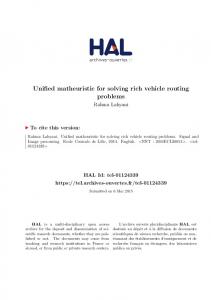
������ �� ����A��A�� � � � � � � A � A��� ���� �A�� � A� � � � A A . . . . . . . �����A� � � � �A�A��� � � A� n3 ? ? ? ? ? ? ? A�� A � A��� � �A� ------ t � � A A�� �A��� n4 n5 n6 n7 n8 n9 �A�A�� (a) � s- - - - - ??????? n1 . . . . . . . n2 ? ? ? ? ? ? ?
4
8 . .. ..... .. ..... 9 .. ..... .. ..... 1 ... .... ... ..... 10 ... .... ... ..... ... ..... .. ..... .. ..... s .. .... t .... .. ..... .. ..... .. . n1 ... .... n9 .. ..... ... n8 .... ... .... ... n7 .. n2 .. .... .... ... n6 n3 .. n5 (b) n4 4
2
Figure 1. An example Layered graph . Lemma 6 [6] For G the configuration network of a line graph G, the optimal S (G )-T (G ) route corresponds to an optimal uniform covering route of G.
3.1. Shortest path algorithm for Layered Directed Acyclic Graph An n Layered directed acyclic graph (LDAG) is a graph with vertices lying on layers; the edges will be from nodes at layer i to i +1 only. A simple example of a layered graph is the grid graph as shown in Figure 3.1(a). The LDAG shown in Figure 3.1(a) can be re-drawn as in Figure 3.1(b). The graph has l rows, (n , l) columns and n , 1 layers and maximum number of nodes in any layer is b = min(l; n , l). Edges from nodes at layer i lead to nodes at layer i +1 only. If adjacency list is used for storing the edges, the edges to next level can be stored in an array of length 2b. An element (i; j ) will be in layer (i + j ) and it is in j th position in array if 1 � i + j � l and in position l , i, otherwise. For finding the shortest path between s and t the vertices in alternate layers will be removed and the number of levels in each iteration reduces by half. Hence, the algorithm will take O(log n) iterations. If there is an edge from nodes ‘x’ at level i , 1 to node ‘y ’ at level i, and if there is another edge from node ‘y ’ to node ‘z ’ at level i + 1, then the two edges can be replaced by a single edge from node ‘x’ to node ‘z ’ with new weight as sum of the weights of original edges. We can find the shortest path in O(log n � log b) time, with O(nb2 = log b) processors on a CREW PRAM and in O(log n � log log b) time with O(nb2 = log log b) processors on a common-CRCW PRAM [11].
3.2. Parallel algorithms for dSVRPTW-line problem An O(n) time Optimal parallel algorithm when the vehicle starts at time 0 can be obtained by first constructing the LDAG for the given problem instance and then for n + 1 iterations, serially in turn removing all nodes in the second layer (the nodes adjacent to source).
For removing nodes at second layer, we allocate one processor to every node in third layer and find the shortest path from source node to that node. Since, the in-degree of any node in LDAG is 2, the number of paths from source node to any node in third layer is 2. So, we can find the shortest path from source node to any node in third layer in O(1) time. Since, there can be at most n + 1 nodes in third layer in any iteration (the maximum number of nodes in any layer before first iteration is n + 1), we need n processors in each iteration. Since, there are n + 1 iterations it we will take O(n) time. Thus, we can find an optimal schedule for coalescing operations when number of jobs is two in O(n) time with O(n2 ) work. We next describe an O(log2 n) time Parallel algorithm. This algorithm computes the optimal path for all vehicle starting times in interval [0; 1). The algorithm is: 1. Construct the LDAG for the given problem instance 2. for t = 0 to log n + 1 do /* log n iterations */ for i = 2 to (n + 1)=2t , 1 pardo if i is even then remove nodes at layer i; The algorithm for removing all nodes at layer i is given below. Here, d is the maximum in-degree (or out-degree) of any node in the current iteration. Clearly, d � n + 1. for each node r of layer i + 1 do /* at most 2b + 1 */ for each node v at layer i incident from r do /* at most d */ for each node p of layer i , 1 incident from v do /* at most d */ parbegin v = compose(Tr;v ; Tv;p ) (a) Tr;p v) (b) Tr;p = minv (Tr;p parend; Lemma 7 The maximum degree of any node before k th iteration will be min(2k ; 2b + 1) Proof: Any node in the graph has degree less than or equal to the degree of source node. This is because, the source node satisfies the same constraints as any other nodes in the graph. So, it is enough if we prove that the degree of source as min(2k ; 2b + 1) in k th iteration. It is evident from algorithm that after every iteration the number of layers decreases by a factor of 2. After every iteration layer i will become layer (i + 1)=2 (if i is odd). Therefore, before kth iteration the layer adjacent to first layer (second layer) will be same as the layer 2k,1 + 1 before the first iteration. (This can be proved by simple induction). The number of nodes layer i before first iteration is 2(i , 1). Therefore, the number nodes in second layer after k iterations will be 2(2k,1 ) = 2k . It is evident from description of our graph that every node is reachable from the source (this implies that every node in the second layer is connected to source) and the maximum number of nodes in any layer is at most
2b + 1 so,
the degree of a node before any iteration can not exceed 2n + 1. Therefore, the degree of source node is min(2k ; 2b +1) in kth iteration. Thus, the result follows.
Lemma 8 For removing nodes at layer i in k th iteration, our algorithm on a CREW PRAM requires , k ) � (log n))� time using (2b + 1) � O log(min(2 b + 1 ; 2 � �
min(2b+1;2k )2 �n log min(2b+1;2k )�log n processors.
Proof:
For removing nodes at layer
i we need to find
Tr;p where, r 2 layer i , 1 and p 2 layer i + 1. For v where, v 2 finding Tr;p we need to find minimum of Tr;p
layer i and r is incident on v , v incident on p. If d is the degree of r then we need to compose d tables and find minimum among these d tables. By Lemma 3 and 4, we can compose two tables or find minimum of two tables in O(log n) time with n=log n processors. We can compose d pairs of tables into d tables in O(log d � log n) time with d � n=(log d � log n) processors. We can also find minimum of d tables in O(log d � log n) time with d � n=(log d � log n) processors. Therefore, we can find Tr;p in O(log d � log n) time with d � n=(log d � log d) processors on a CREW PRAM. Since, there can be d nodes in layer i + 1 associated with v and at most (2b + 1) nodes in layer i , 1 the number of processors for removing nodes at layer i is (2b + 1) � d � (d=log d) � (n=log n). We have by Lemma 7 that the degree of any node before k th itk eration , is min(2b + 1; 2 ). Therefore, we need O(2b + �
1) � (min(2b + 1;,2k )2 =log min(2b + 1; 2k )) � (�n=log n) processors and O log(min(2b + 1; 2k ) � log n) time for
kth iteration.
Theorem 3 There is a CREW PRAM algorithm for dSVRPTW-line that takes O(log2 n � log b) time using n2 b2 =log b � log n processors. Proof: The initial number of layers in the graph is n +1. In every iteration we will be removing half of layers present. Therefore, there will be (n + 1)=2k layers in k th iteration. th Combining this with � Lemma 8, kIf 2in k � iteration we use , n+1 � min(2 b +1 ; 2 ) � n 2k � (2b + 1) � log min(2b+1;2k )�log n processors, time ,
�
will be O log min(2b + 1; 2k ) . These expressions will be maximum when 2k � 2b + 1 or when k � log(2b + 1). Therefore, the maximum number of processors in any iteration is n2 b2 =log b � log n. Since each iteration takes at most O (log n � log b) time and there are log n + 1 iterations, the time required for our algorithm is O(log2 n � log b). Thus the result follows.
4. Travelling Repairman Problem Afrati et. al. [1] have an O(n2 ) algorithm for special case of travelling repairman problem when handling time
is zero and all the locations are in a line without having time windows associated with them. (see Tsitsiklis [13]) We first describe a simple O(n2 ) time dynamic programming algorithm for this problem. We can fix any instance G of TRP-line to be ordered in the form am ; am,1 ; : : : ; a1 ; D; b1 ; : : : ; bp . We assume that nodes a0 and b0 , both refer to same node, the central depot D from where the vehicle originates and terminates. Since all locations are on a line there are edges between two consecutive locations only. Cost of an edge is time taken for the vehicle to travel between the two locations. If S = v1 ; : : : ; vm+p+1 is an optimal feasible route that covers G, then S is uniform if for any k � m + p + 1; v1 ; : : : ; vk is an optimal feasible route that covers the subgraph of G induced by ai ; ai,1 ; : : : ; a1 ; D; b1 ; : : : ; bj for some i and j such that k = i + j + 1. If v1 ; : : : ; vm+p+1 is a uniform route in G, then the subsequence v1 ; : : : ; vk can be represented by the ordered pair (i; j ) where ai and bj both appear in this subsequence and i + j + 1 = k; subsequence v1 ; : : : ; vk ; vk+1 is represented by either (i + 1; j ) or (i; j + 1) depending on whether vk+1 is ai+1 or bj +1 . In general, for 0 � i � m and 0 � j � p, let C (i; j ; L) (respectively C (i; j ; R)) be the cost of uniform route on network induced by the subgraph ai ; : : : ; a1 ; D; b1 ; : : : ; bj in which ai is the last element of the sequence (bj is the last element respectively) and let T (i; j ; L) and T (i; j ; R) be the times taken for these uniform routes. The initial conditions for the dynamic programming algorithm is C (0; 0; L) = C (0; 0; R) = T (0; 0; L) = T (0; 0; R) = 0. For i; j > 0, let � = T (i; j , 1; L) + t(i; j ), = T (i; j , 1; R) + t(j , 1; j ), = T (i + 1; j ; L) + t(i; i + 1) and � = T (i + 1; j ; R) + t(i; j ). Then
C (i; j; R) = minfC (i; j , 1; L) + �; C (i; j , 1; R) + g C (i; j; L) = �minfC (i + 1; j; R) + ; C (i + 1; j; L) + �g ) = C (i; j , 1; L) + � T (i; j; R) = � ifif CC ((i;i; j;j; R R ) = C (i; j , 1; L) + �
if C (i; j ; L) = C (i + 1; j ; R) + T (i; j; L) = � if C (i; j ; L) = C (i + 1; j ; L) + �
Theorem 4 The special case of Line-TRP in which the handling times of all nodes is zero can be solved in O(n2 ) where n is the number of locations. Proof: The algorithm proceeds by computing C (i; j; L) and C (i; j; R) for 0 � i � m and 0 � j � p. Each value of C can be computed in constant time using above given equations. Since there are O(n2 ) values to be computed, the theorem follows. We construct a configuration network for a given instance graph G with nodes representing uniform routes in G and edges representing extensions of one route to another by the addition of one new node; configuration network is again a LDAG. The construction is very similar to
one in the dSVRPTW-line problem. The vertices in configuration network are V = f(i; j; R); (i; j; L) : 1 � i � m; 1 � pg[ f(0; 0; D)g [ f(m + 1; p + 1; D)g with source as S (G ) = (0; 0; D) and sink as T (G ) = (m + 1; p + 1; D) respectively. Each (u; v ) in the graph denotes optimal cost route between the vertices u and v . We associate three values d(u; v ), a(u; v ) and len(u; v ) with each edge. let u; u1; u2; : : : ; ul ; v be the optimal cost route between the vertices then d(u; v ) denotes the sum of waiting times of nodes in that path i.e., d(u; v ) = (l + 1) � t(u; u1 ) + l � t(u1 ; u2)+: : :+2�t(ul,1; ul )+t(ul ; v), a(u; v) denotes the travelling time from u to v in the optimal path i.e., a(u; v ) =
t(u; u1)+ t(u1 ; u2)+ t(u2 ; u3)+ : : : + t(ul,1 ; ul )+ t(ul ; v) len(u; v) denotes the length of the optimal path (i.e., l + 1). The initial values of d(u; v), a(u; v), are t(u; v), where t(u; v ) denotes the travel time between those nodes. The initial values of len(u; v ) is 1 if t(u; v ) 6= 0, else, len(u; v) is 0. There are edges from (m; p; L) and (m; p; R) to (m +1; p + 1; D) and from (0; 0; D) to (1; 0; L) and (0; 1; R). Finally, for 1 � i � m and 1 � j � p there are edges from (i; j; L) to (i + 1; j; L), (i; j; L) to (i; j + 1; R), (i; j; R) to (i; j + 1; R) and from (i; j; R) to (i + 1; j; L). The node (i; j; L) denotes the optimal route covering [ai ; bj ] with ai being the last node visited. Similarly the node (i; j; R) denotes the optimal route covering [ai ; bj ] with bj being the last node visited. Node (0; 0; D) and (m + 1; p + 1; D) and
denote the null route and optimal route respectively. There are n + 1 layers in the configuration network G , where n = m + p + 1; (0; 0; D) will be in first layer and (m + 1; p + 1) in the last layer; (i; j; L) and (i; j; R) will be in (i + j + 1)th layer. If b = min(m; p), then the maximum number of nodes in any layer will be 2b + 1. The first layer will have only the source node and the last layer will have only sink node. An O(n) time Optimal parallel algorithm can again be obtained by first constructing the LDAG for the given problem instance and then for n +1 iterations, serially in turn removing all nodes in the second layer. For removing nodes at second layer we use the same algorithm as for dSVRPTWproblem. An O(log2 n) time parallel algorithm for TRP-line problem can again be obtained by first constructing a LDAG for the given problem instance and then for log n iterations removing nodes in even layers. The algorithm for removing all nodes at layer i is given below. Here, d is the maximum in-degree (or out-degree) of any node in the current iteration. Clearly, d � 2n + 1. for each node r of layer i , 1 do /* at most 2b + 1 */ for each node v at layer i incident from r do /* at most d */ for each node p of layer i + 1 incident from v do /* at most
d */ parbegin (a) d(r; p) = minv (d(r; v ) + d(v; p) + len(v; p) � a(r; v )) (b) Let u be the node that gives rise to the minimum value of d(r; p) (c) a(r; p) = a(r; u) + a(u; p) (d) len(r; p) = len(r; u) + len(u; p) parend; The correctness proof will be similar to that for dSVRPTW-line problem. The algorithm takes O(log n � log b) time with O(nb2 = log b) processors on a CREW PRAM where b = min(m; p). Acknowledgements: We wish to thank anonymous referees for suggesting valuable corrections and for pointing out typos.
References [1] F. Afrati, A. Cosmadakis, C. H. Papadimitriou, and N. Papakonstantinou. The complexity of the traveling repairman problem. Theory of Information Applications, 20(1):79–87, 1986. [2] R. K. Ahuja, T. L. Magnanti, and J. D. Orlin. Network Flows. Prentice-Hall Englewood Cliffs, 1993. [3] L. Bodin, B. Golden, A. Assad, and M. Ball. Routing and scheduling of vehicles and crews: The state of the art. Computer Operations Research, 10:62–212, 1983. [4] M. L. Fredman and R. E. Trajan. Fibonacci heaps and their uses in improved network optimization algorithms. J. ACM, 34(3):596–615, 1987. [5] M. R. Garey and D. S. Johnson. Two-processor scheduling with start times and deadlines. SIAM Journal of Computing, 6:416–426, 1977. [6] A. Gupta and R. Krishnamurti. Parallel algorithms for vehicle routing problems. In Proceedings of High Performance Computing, pages 144–151. IEEE, 1997. [7] J. K. Lenstra, A. H. G. R. Kan, and B. Brucker. Complexity of machine scheduling problems. Annals of Discrete Mathematics, 1:343–362, 1977. [8] C. H. Papadimitriou. The euclidean traveling salesman problem is P -complete. Theoretical Computer Science, 4:237–244, 1977. [9] H. Psaraftis, M. Solomon, T. Magnanti, and T. Kim. Routing and scheduling on a shoreline with release times. Management Science, 36(2):254–265, 1987. [10] M. W. P. Savelsbergh. Local search in routing problems with time windows. Annals of Operation Research, 4:285–305, 1985/6. [11] S. Saxena. Design and Analysis of Some Combinatorial and Computational Geometry Problems for Parallel Execution. PhD thesis, Comp. Sci. & Engg., IIT Delhi, January 1989. [12] M. Solomon and J. Desrosiers. Time window constrained routing and scheduling problems: A survey. Transportation Science, 22:1–13, 1988. [13] J. N. Tsitsiklis. Special cases of traveling salesman and repairman problems with time windows. Networks, 22:263– 282, 1992.
N