Parallel Graph Narrowing Rachid Echahed and Jean-Christophe Janodet 46, avenue Felix Viallet 38031 Grenoble - France
[email protected] Abstract We investigate graph narrowing as the operational semantics of functional logic programming languages. We mainly show and discuss how weakly needed narrowing as well as parallel narrowing may be extended to graph structures.
1
Introduction
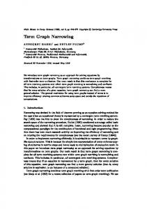
Functional logic programming languages integrate, in a uniform way, functional languages and logic languages. The resulting languages (e.g., [12, 13]) have the advantages of both paradigms. Their operational semantics is often based on firstorder term narrowing (see [11]). However, in practice, data structures are not always represented as first-order terms but rather as cyclic graphs. Hence, several declarative languages such as Haskell, Clean or Life allow to work with graphs explicitely. There are many reasons which motivate the use of graphs. They allow to go beyond the processing of first-order terms by handling efficiently real-wold data types represented as complex cyclic graphs. They also permit the sharing of subexpressions which leads to efficient computations. Consider, for instance, the rule R = O+Z → Z. In Fig. 1, the length of the first (term) narrowing derivation is 2p − 1 whereas the length of the second (graph) narrowing derivation is p. In practice, many programming languages are constructor-based, i.e., operators called constructors which are used to build the data structures are distinguished from operators called defined functions which are defined by means of rewrite rules. In this paper, we follow this discipline and study the narrowing relation induced by the so-called weakly admissible graph rewriting systems (WAGRSs) [8]. Actually, using graph rewriting systems instead of term rewriting systems is not an easy task. The classical properties of term rewriting systems such as confluence or the completeness of the narrowing relation cannot be lifted without caution to graph rewriting systems (see [6, 10]). Therefore, WAGRSs have been tailored so that they preserve the wanted properties. Moreover, WAGRSs extend the constructor-based weakly orthogonal term rewriting systems [3]. In this setting, efficient narrowing strategies have been proposed such as (weakly) needed narrowing [2, 3] and parallel narrowing [3]. In this paper, we show that (weakly) needed narrowing and parallel narrowing can be extended to the framework of WAGRSs. In the following section, we give briefly some preliminaries. Section 3 defines the WAGRSs and the sequential and parallel rewrite relations they induce. Most general narrowing and weakly needed narrowing are defined in Section 4 where we
+ + p+1
+
+
+
+
+ X
...
+ X
X
X n0:+
+ X
X
+
;[np−1 , R, {X7→q:O}]
...
+
O X
O
+
+
+ X
2p −2 ; [Id]
+
;[1p−1 , R, {X7→O}]
O
O
+ O
n0:+
n1:+
n1:+
np−1 :+
q:O
+ O
O
O
p−1 ; [Id]
q:O
p+1
np :X
Figure 1: establish their completeness. Section 5 is devoted to parallel graph narrowing. We conclude the paper in Section 6.
2
Definitions and Notations
Many different notations are used in the literature to investigate graph rewriting [9, 15, 16]. The aim of this section is to give briefly some key definitions in order to make easier the understanding of the paper. We are mostly consistent with [5]. We consider a graph as a set of nodes and edges between the nodes. Each node is labeled with an operation symbol or a variable. Let Σ = hS, Ωi be a many-sorted signature, X a set of variables and N a set of nodes. A graph g over hΣ, N , X i is a tuple g = hNg , Lg , Sg , Rootsg i such that Ng is a set of nodes, Lg : Ng → Ω ∪ X is a labeling function which maps to every node of g an operation symbol or a variable, Sg is a successor function which maps to every node of g a (possibly empty) string of nodes and Rootsg is a set of distinguished nodes of g, called its roots. We also assume three conditions of well definedness. (1) Graphs are well typed : a node n is of the same sort as its label Lg (n), and its successors Sg (n) are compatible with the rank of Lg (n). (2) Graphs are connected : for all nodes n ∈ Ng , there exist a root r ∈ Rootsg and a path from r to n. (3) Let Vg be the set of variables of g. For all x ∈ Vg , there exists one and only one node n ∈ Ng such that Lg (n) = x. A term graph is a (possibly cyclic) graph with one root denoted Rootg . Two . term graphs g1 and g2 are bisimilar, denoted g1 = g2 , iff they represent the same (infinite) tree when one unravels them [4]. We write g1 ∼ g2 when the term graphs g1 and g2 are equal up to renaming of nodes. As the formal definition of graphs is not useful to give examples, we introduce a linear notation [5]. In the following grammar, the variable A (resp. n) ranges over the set Ω ∪ X (resp. N ) : Graph ::= Node | Node + Graph Node ::= n:A(Node,. . . ,Node) | n
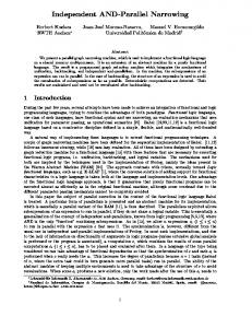
The set of roots of a graph defined with a linear expression contains the first node of the expression and all the nodes appearing just after a +. Example 2.1 In Fig. 2, we give two examples of graphs denoted G and T . The term graph G is given by (1) NG = {n1, . . . , n5}, (2) RootG = n1, (3) LG is defined by LG (n1) = LG (n5) = c, LG (n2) = g, LG (n3) = s and LG (n4) = a and (4) SG is defined by SG (n1) = n2.n5 , SG (n2) = n3.n3 , SG (n3) = n4, SG (n4) = ε and SG (n5) = n3.n1, thus G = n1:c(n2:g(n3:s(n4:a),n3),n5:c(n3,n1)). On the other hand, T is a graph with two roots {l1,r1} representing a rewrite rule (see Def. 3.1) : T = l1:g(l2:s(l3:u),l4:s(l5:v)) + r1:s(r2:g(l3,l4)). n1:c
n5:c
n2:g
l1:g
r1:s
n3:s
l2:s
l4:s
n4:a
l3:u
l5:v
G
r2:g
T
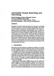
Figure 2: A subgraph of a graph g rooted by a node p, denoted g|p , is built by considering p as a root and deleting all the nodes which are not accessible from p in g (e.g., G|n2 = n2:g(n3:s(n4:a),n3) in Fig. 2). The sum of two graphs g1 and g2 , denoted g1 ⊕g2 , is the graph whose nodes and roots are those of g1 and g2 and whose labeling and successor functions coincide with those of g1 and g2 . A multiple pointer redirection ρ from the nodes p1 , . . . , pn to the nodes q1 , . . . , qn is a function ρ : N → N such that ρ(pi ) = qi for all i ∈ 1..n and ρ(p) = p for all nodes p such that p 6= p1 , p 6= p2 , . . . and p 6= pn . Given a graph g and a pointer redirection ρ = {p1 7→ q1 , . . . , pn 7→ qn }, we define ρ(g) as the graph whose nodes and labeling function are those of g, whose successor function satisfies Sρ(g) (n) = ρ(n1 ) . . . ρ(nk ) if Sg (n) = n1 . . . nk for some k ≥ 0 and whose roots are Rootsρ(g) = {ρ(n1 ), . . . , ρ(nk )} ∪ {n1 , . . . , nk } if Rootsg = {n1 , . . . , nk }. Given two term graphs g and u and a node p of the same sort as Rootu , we define the replacement by u of the subgraph rooted by p in g, denoted g[p ← u], in three stages : (1) Let H = g ⊕ u. (2) Let ρ be the pointer redirection from p to Rootu , H 0 = ρ(H) and r = ρ(Rootg ). (3) g[p ← u] = H 0 |r . Example 2.2 Let G be the term graph of Example 2.1 and D = r1:s(r2:g(n4:a,n3:s(n4))). The sum G ⊕ D is given by n1:c(n2:g(n3:s(n4:a),n3),n5:c(n3,n1)) + r1:s(r2:g(n4,n3)) (see Fig. 3). Let ρ be the pointer redirection such that ρ(n2) = r1 and ρ(p) = p for all p 6= n2. The graph ρ(G⊕D) is defined by n1:c(r1:s(r2:g(n4:a,n3:s(n4)),n5:c(n3,n1)) + n2:g(n3,n3). Thus the replacement by D of the subgraph rooted by n2 in G is G[n2 ← D] = n1:c(r1:s(r2:g(n4:a,n3:s(n4)),n5:c(n3,n1)). A (rooted) homomorphism h from a graph g1 to a graph g2 , denoted h : g1 → g2 , is a mapping from Ng1 to Ng2 such that Rootsg2 = h(Rootsg1 ) and for all nodes / X then Lg2 (h(n)) = Lg1 (n) and Sg2 (h(n)) = h(Sg1 (n)) and if n ∈ Ng1 , if Lg1 (n) ∈ Lg1 (n) ∈ X then h(n) ∈ Ng2 . If h : g1 → g2 is a homomorphism and g is a subgraph
n1:c r1:s
n5:c
n2:g
r2:g
n1:c r1:s
n3:s
r2:g
n4:a
n5:c
n2:g n3:s n4:a G[n2 ← D]
G⊕D
Figure 3: of g1 rooted by p, then we write h(g) for the subgraph g2 |h(p) . If h : g1 → g2 is a homomorphism and g is a graph, h[g] is the graph built from g by replacing all the subgraphs shared between g and g1 by their corresponding subgraphs in g2 . A term graph l matches a graph g at node n if there exists a homomorphism h : l → g|n . h is called the matcher of l on g at node n. Two term graphs g1 and g2 are unifiable iff there exist two graphs G and H and a homomorphism h : G → H such that (1) g1 and g2 are both subgraphs of G and (2) h(g1 ) = h(g2 ). h is called a unifier of g1 and g2 . If g1 and g2 are unifiable, we can prove that there exists a most general unifier in the following sense : there exist a graph g and a homomorphism h : (g1 ⊕ g2 ) → g such that (1) h(g1 ) = h(g2 ) = g and (2) for all unifiers h0 : G → H, there exists a homomorphism φ : g → h0 (g1 ⊕ g2 ). Example 2.3 Consider the subgraph G|n2 of Example 2.1, let L = l1:g(l2:s(l3:u),l4:s(l5:v)) and µ the mapping from NL to N(G
such that n2 ) µ(l1) = n2, µ(l2) = µ(l4) = n3 and µ(l3) = µ(l5) = n4. µ is a homomorphism from L to G|n2 , thus L matches G at node n2. On the other hand, let R = r1:s(r2:g(l3:u,l4:s(l5:v))). R and L share the subgraphs l3:u and l4:s(l5:v) whose images by µ are respectively n4:a and n3:s(n4:a). Hence µ[R] = r1:s(r2:g(n4:a,n3:s(n4))), i.e., µ[R] is the graph D of Example 2.2. Finally, let L1 = n1:f(n2:a,n3:x) and L2 = m1:f(m2:y,m3:s(m4:a)). L1 and L2 are unifiable since there exist a term graph L3 = p1:f(p2:a,p3:s(p4:a)) and a homomorphism υ : (L1 ⊕ L2) → L3 such that υ(L1) = υ(L2) = L3. |
Independently of homomorphisms, we need substitutions in order to define solutions computed by narrowing. A substitution σ is a partial function from the set of variables X to a set of term graphs. Dσ denotes the domain of σ, i.e., the set of variables x such that σ(x) is not a graph reduced to a single node labeled with the variable x. By Id, we mean any substitution such that D(Id) = ∅. The restriction of σ to a set V of variables, σ|V , is such that D(σ|V ) = V ∩ Dσ and σ|V (x) = σ(x) for all x ∈ D(σ|V ). σ(g) denotes the graph built from g by replacing all the variables x ∈ Dσ by their images σ(x). Applying a substitution on a graph is roughly the same as applying a substitution on a first-order term, except that it preserves the sharing of subgraphs. . Given two term graphs g1 and g2 , we write g1 ≤ g2 iff there exists a substitution . θ such that θ(g1 ) = g2 . The composition of two substitutions σ1 and σ2 is the substitution σ2 ◦ σ1 such that D(σ2 ◦ σ1 ) = Dσ1 ∪ Dσ2 and σ2 ◦ σ1 (x) = σ2 (σ1 (x)) for all x ∈ Dσ1 and σ2 ◦ σ1 (x) = σ2 (x) for all x ∈ (Dσ2 − Dσ1 ). An idempotent substitution satisfies σ ◦ σ = σ. Given two substitutions σ1 and σ2 and. a set V of variables, we say that σ1 is more general than σ2 on V , denoted σ1 ≤ σ2 [V ], if
. there exists a substitution θ such that θ ◦ σ1 (x) = σ2 (x) for all x in V . We write . . . σ1 = σ2 [V ] iff σ1 ≤ σ2 [V ] and σ2 ≤ σ1 [V ]. Finally, let A be a set of substitutions. . We denote by A/ = the “quotient” set which consists of substitution representatives of A up to renaming and bisimilarity. Example 2.4 Let σ(u) = σ(v) = n4:a. The reader may check that σ(L) = l1:g(l2:s(n4:a),l4:s(n4)). Let σ 0 = {x 7→ m1:b(m2:u,n4:a)}. Then, (σ ◦ σ 0 )|{x,u} = {x 7→ m1:b(n4:a,n4), u 7→ n4:a}.
3
Weakly Admissible Graph Rewriting Systems
This section introduces briefly the graph rewriting systems (GRSs) we consider (see [8] for details). Let Σ = hS, C, Di be a constructor-based signature [14]. In Example 2.1, we assume that c, s and a are constructors (∈ C) and g is a defined operation (∈ D). A functional node (resp. constructor node, variable node) is a node labeled with a defined operation (resp. constructor, variable). In this paper, we investigate graph narrowing for the class of what we call admissible term graphs (atg) [8]. Roughly speaking, an atg corresponds, according to the imperative point of view, to nested procedure (function) calls whose parameters are complex constructor cyclic graphs (i.e., classical data structures). Definition 3.1 A term graph g is an admissible term graph (atg) if there exists no path from a functional node of g to itself. An atg is a pattern if it has a tree structure (i.e., linear first-order term) which has one and only one defined operation at its root. A constructor graph is a graph with no functional node. A rewrite rule is a graph with two roots, denoted l → r, such that (1) l is a pattern (thus an atg), (2) r is an atg, (3) l is not a subgraph of r and (4) Vr ⊆ Vl . We say that two rules l1 → r1 and l2 → r2 overlap iff their left-hand sides are unifiable. In Fig. 2, G is an atg and T is a rewrite rule. As for z:g(z,z) and z:g(n:s(z),n), they are not atgs since g is a defined operation which belongs to a cycle. Condition (3) in the definition of rewrite rule is necessary to prove the stability of the set of atgs w.r.t. the rewrite relation [8]. Definition 3.2 A weakly admissible graph rewriting system (WAGRS) is a pair SP = hΣ, Ri where Σ is a constructor-based signature and R is a set of rewrite rules such that if two rules l1 → r1 and l2 → r2 of R overlap, then their instantiated righthand sides are equal up to renaming of nodes, i.e., if there exist a graph g and a homomorphism h : (l1 ⊕ l2 ) → g such that h(l1 ) = h(l2 ) = g, then h[r1 ] ∼ h[r2 ]. Example 3.3 The following set of rules defines a WAGRS : (R1) (R2) (R3) (R4) (R5) (R6) (R7)
l1:f(l2:a,l3:x) l1:f(l2:x,l3:s(l4:y)) l1:g(l2:a,l3:a,l4:x) l1:h(l2:a) l1:i(l2:a,l3:x,l4:y) l1:i(l2:x,l3:a,l4:y) l1:i(l2:x,l3:y,l4:a)
-> -> -> -> -> -> ->
r1:d(r1,l3:x) r1:d(r1,r2:s(r3:a)) l4:x l2:a r1:a l2:x l2:x
Indeed, the rules R1 and R2 (resp. R5, R6 and R7) overlap and their instantiated right-hand sides are equal up to renaming of nodes.
Below, we recall the definition of a graph rewriting step [5]. Definition 3.4 Let g1 be an atg, g2 a graph, R a rewrite rule and p a node of g1 . A rewriting step from g1 to g2 at node p using the rule R is defined by g1 →[p, l→r] g2 iff there exist a variant l → r of R and a homomorphism h : l → g1 |p (i.e., l matches g1 at node p) such that g2 = g1 [p ← h[r]]. In this case, g1 |p is called a redex of g1 ∗
rooted by p. → denotes the reflexive and transitive closure of →. In [8], we have proved that the rewrite relation is confluent (and confluent modulo the bisimilarity) w.r.t. atgs and WAGRSs. Example 3.5 According to Example 2.3, L matches G at node n2 with homomorphism µ and µ[R] = r1:s(r2:g(n4:a,n3:s(n4))). We infer that G[n2 ← µ[R]] = n1:c(r1:s(r2:g(n4:a,n3:s(n4))),n5:c(n3,n1)), since µ[R] is the atg D of Example 2.2. Let G0 be this last graph. By Definition 3.4, G →[n2, L→R] G0 . We now introduce parallel graph rewriting over admissible graphs. If parallel rewriting can be easily conceived in the framework of first-order terms, this is unfortunately not the case when one deals with graph structures. The main difficulty comes from the sharing of subgraphs. The reader may find more details in [8]. Definition 3.6 Let g1 be an atg, g2 a graph, p1 , . . . , pn n distinct nodes of g1 and R1 , . . . , Rn n rewrite rules. A parallel rewriting step from g1 to g2 at nodes p1 , . . . , pn using the rules R1 , . . . , Rn , denoted g1 −→ bb [p1 , R1 ]...[pn , Rn ] g2 , is given by : 1. Let li → ri be a variant of Ri and hi : li → g1 |pi for all i ∈ 1..n. 2. Let H = g ⊕ h1 [r1 ] ⊕ . . . ⊕ hn [rn ]. 3. Let ρ1 , . . . , ρn be the pointer redirections such that for all i ∈ 1..k, ρi (pi ) = Roothi [ri ] and ρi (p) = p for all nodes p such that p 6= pi . 4. Let ρ = ρµ(1) ◦ . . . ◦ ρµ(n) where µ : 1..n → 1..n is a permutation such that if i < j, then there exists no path from pµ(i) to pµ(j) . 5. Let H 0 = ρ(H) and r = ρ(Rootg ). 6. g2 = H 0 |r . Condition (4) in the previous definition can always be fulfilled. Its rˆ ole is to take into account the relative positions of the different redexes to be transformed so that the parallel rewrite relation −→ bb can be simulated by the rewrite relation → (i.e., if ∗ g1 −→ bb g2 then g1 → g2 ). Example 3.7 Let g = p1:d(p2:u(p3:a),p4:v(p2)) be an atg and l1 → r1 and l2 → r2 two rules such that l1 = l1:u(l2:x), r1 = r1:s(l2:x), l2 = l3:v(l4:y) and r2 = l4:y. l1 matches g at node p2 using the homomorphism h1 : l1 → g|p2 and h1 [r1 ] = r1:s(p3:a). On the other hand, l2 matches g at node p4 using the homomorphism h2 : l2 → g|p4 and h2 [r2 ] = p2:u(p3:a). Let H = g ⊕ h1 [r1 ] ⊕ h2 [r2 ] = p1:d(p2:u(p3:a),p4:v(p2)) + r1:s(p3) + p2. (see Fig. 4). Let ρ1 = {p2 7→ r1} and ρ2 = {p4 7→ p2}. There exists a path from p4 to p2 in g but none from p2 to p4. So we define ρ = ρ1 ◦ ρ2 = {p2 7→ r1, p4 7→ r1}. The reader may check that ρ(H) = H 0 = p1:d(r1:s(p3:a),r1) + r1 + p2:u(p3) + p4:v(r1) and ρ(Rootg ) = p1. Hence, by Def. 3.6, g −→ bb [p2, l1 →r1 ][p4, l2 →r2 ] g2 where g2 = p1:d(r1:s(p3:a),r1).
p1:d r1:s
p2:u
p1:d p4:v
p3:a
r1:s
p2:u
p4:v
p3:a H0
H
Figure 4:
4
Weakly Needed Graph Narrowing
In this section, we define graph narrowing and extend weakly needed term narrowing [3] to graphs. Roughly speaking, a graph g2 is obtained from a graph g1 by means of graph narrowing iff there exists a substitution σ such that σ(g1 ) rewrites into g2 : Definition 4.1 Let g1 be an atg, R a rewrite rule, p a non variable node of g1 , σ a substitution and g2 a graph. A narrowing step from g1 to g2 at node p using the rule R and the substitution σ is defined by g1 ;[p, R, σ] g2 ⇐⇒ σ(g1 ) →[p, R] g2 . In this paper, we deliberately use substitutions within narrowing steps instead of homomorphisms [6] for a better readability. Such a substitution may be, for instance, the most general unifier of g|p w.r.t. the left-hand side of R : We say that an atg g is unifiable w.r.t. a pattern l iff there exist an idempotent substitution σ and a homomorphism h : (g⊕l) → σ(g) such that h(g) = h(l) = σ(g). σ is called a unifier of g w.r.t. l. We say that σ is a most general unifier of g w.r.t. l iff (1) σ is a unifier of g w.r.t. l, (2) the homomorphism h : (g ⊕ l) → σ(g) is a most . general unifier of g and l and (3) σ ≤ η for all unifiers η of g w.r.t. l. Example 4.2 Let H = n1:c(n2:g(n3:x,n3),n4:c(n3,n1)) and L → R the rule represented in Fig. 2. We claim that H|n2 is unifiable w.r.t. L. Indeed, let σ = {x 7→ m1:s(m2:z)}. Then, σ(H) = n1:c(n2:g(m1:s(m2:z),m1),n4:c(m1,n1)) and there exists a homomorphism υ from (H|n2 ⊕ L) to σ(H|n2 ) such that υ(n2) = υ(l1) = n2, υ(n3) = υ(l2) = υ(l4) = m1 and υ(l3) = υ(l5) = m2. The reader may check that if H1 = n1:c(p1:s(p2:g(m2:z,m1:s(m2))),n4:c(m1,n1)), then σ(H) →[n2, L→R] H1 . So we conclude that H ;[n2, L→R, σ] H1 . Narrowing is used to solve goals. A solution of a goal is often represented by a substitution. We say that a substitution σ is computed by a narrowing deriva∗ tion from an atg g1 to an atg g2 and write g1 ;σ g2 iff there exists a derivation g1 ;[p1 , l1 →r1 , σ1 ] . . . ;[pk , lk →rk , σk ] g2 and σ = (σk ◦ . . . ◦ σ1 )|Vg1 . Example 4.3 Let H ;[n2, L→R, σ] H1 be the narrowing step of Example 4.2. Consider a second narrowing step starting with H1 and the rule L0 → R0 where L0 = l1:g(l2:a,l3:w) and R0 = l3:w. H1 |p2 and L0 unify and an m.g.u. of H1 |p2 w.r.t. L0 is σ 0 = {z 7→ m3:a}. Therefore, H1 ;[p2, L0 →R0 , σ0 ] H2 where H2 = ∗
n1:c(p1:s(m1:s(m2:z)),n4:c(m1,n1)). Hence, H ;θ H2 with θ = (σ 0 ◦ σ)|VH = {x 7→ m1:s(m3:a)}. Below, we recall the notions of soundness and completeness of narrowing. These definitions do not consider narrowing as an inference rule for solving some particular goals but rather as a general computational model for arbitrary expressions
(graphs). The traditional goals such as equations can be represented as boolean expressions. Definition 4.4 We say that the narrowing relation ; is sound iff for all atgs g, ∗ constructor graphs c and substitutions θ such that g ;θ c, there exists a constructor ∗ . graph s such that θ(g) → s and s = c. We say that the narrowing relation ; is complete iff for all atgs g, constructor graphs c and constructor substitutions θ ∗ such that θ(g) → c, there exist a constructor graph s and a substitution σ such that . . ∗ g ;σ s, s ≤ c and σ ≤ θ [Vg ]. In [6], we have established that most general narrowing ; is sound and complete. ¯ which extends We now define a sequential graph narrowing strategy, denoted Λ, weakly needed term narrowing [3] to atgs. A sequential graph narrowing strategy, ¯ is a partial function which takes an atg g and returns a set of tuples of e.g. Λ, the form (p, R, σ) such that g ;[p, R, σ] g 0 for some atg g 0 . We write g ;Λ¯ g 0 iff ¯ g ;[p, R, σ] g 0 and (p, R, σ) ∈ Λ(g). ¯ is based on the organization of WAThe sequential graph narrowing strategy Λ GRSs as forests of definitional trees. A definitional tree [1] is a hierarchical structure whose leaves are the rules of a WAGRS used to define some operation. In the following definition, branch and rule are uninterpreted symbols, used to construct the nodes of a definitional tree. Definition 4.5 A tree T is a partial definitional tree, or pdt, with pattern π iff one of the following cases holds : • T = rule(π → r), where π → r is a variant of a rule of R. • T = branch(π, o, T1 , . . . , Tk ), where o is a variable node of π, o is of sort s, c1 , . . . , ck (k > 0) are different constructors of the sort s and for all j ∈ 1..k, Tj is a pdt with pattern π[o ← p : cj (o1 : X1 , . . . , on : Xn )], such that n is the number of arguments of cj , X1 , . . . , Xn are new variables and p, o1 , . . . , on are new nodes. We write pattern(T ) to denote the pattern argument of T . A definitional tree T of an operation f is a finite pdt with a pattern of the form p : f (o1 : X1 , . . . , on : Xn ) where n is the number of arguments of f , X1 , . . . , Xn are new variables and p, o1 , . . . , on are new nodes. A forest of definitional trees (fdt) F of an operation f is a set of definitional trees such that every rule defining f appears in one and only one tree in F. Example 4.6 Consider the WAGRS of Example 3.3. A definitional tree Tg of the operation g is represented in Fig. 5 and formally defined by : Tg = branch(k1:g(k2:X1,k3:X2,k4:X3), k2, branch(k1:g(k5:a,k3:X2,k4:X3), k3, rule(k1:g(k5:a,k6:a,k4:X3) → k4:X3))) Notice that the rules R1 and one definitional tree. This is we represent possible fdts Ff {Ti1 , Ti2 , Ti3 } corresponding to
R2 of Example 3.3 cannot be represented in only why we introduced the notion of fdts. In Fig. 5, = {Tf1 , Tf2 }, Fg = {Tg }, Fh = {Th } and Fi = the operations f, g, h and i.
k1:i(k2:X1,k3:X2,k4:X3)
k1:i(k2:X1,k3:X2,k4:X3)
k1:i(k2:X1,k3:X2,k4:X3)
k1:i(k5:a,k3:X2,k4:X3)
k1:i(k2:X1,k5:a,k4:X3)
k1:i(k2:X1,k3:X2,k5:a)
k6:a
k2:X1
k2:X1
Ti1
Ti2
Ti3
k1:g(k2:X1,k3:X2,k4:X3)
k1:f(k2:X1,k3:X2)
k1:f(k2:X1,k3:X2)
k1:h(k2:X1)
k1:g(k5:a,k3:X2,k4:X3)
k1:f(k4:a,k3:X2)
k1:f(k2:X1,k4:s(k5:X3)
k1:h(k3:a)
k1:g(k5:a,k6:a,k4:X3)
k5:d(k5,k3:X2)
k6:d(k6,k7:s(k8:a)
k3:a
k4:X3
Tf1
Tf2
Th
Tg
Figure 5: ¯ is a partial function that operates Our sequential graph narrowing strategy Λ ¯ on atgs in the presence of WAGRSs. Λ(g) returns, when it is possible, a set of tuples (n, l → r, σ) such that g is narrowable at node n using the rule l → r and the substitution σ. σ is a particular unifier of g|n w.r.t. l, which is generally not a most general unifier of g|n w.r.t. l. Actually, σ may assign some variables of g which are ¯ which takes two arguments : an ¯ uses an auxiliary function λ not variables of g|n . Λ operation-rooted atg and a pdt of this operation. ¯ is the partial function such that Definition 4.7 Let g be an atg. Λ ¯ ¯ ¯ Λ(g) = λ(g|p , T1 ) ∪ . . . ∪ λ(g|p , Tn ) where p is the leftmost-outermost functional node of g and {T1 , . . . , Tn } is an fdt of the label of p in g. Let g be an operation-rooted atg and T a pdt such that pattern(T ) unifies g at the ¯ T ) is a set of triples of the form (p, R, σ), where p is a non variable node root. λ(g, of g, R is a rewrite rule and σ is a unifier of g|p w.r.t the left-hand side of R. ¯ T ) is defined as the smallest set such that : λ(g, {(p, R, σ)} if T = rule(π → r), p = Rootg , R = π → r and σ is a most general unifier of g w.r.t. π ; ¯ Ti ) λ(g, if T = branch(π, o, T1 , . . . , Tk ) and g and pattern(Ti ) unify for some i ∈ 1..k ; {(p, R, σ)} if T = branch(π, o, T1 , . . . , Tk ), ¯ T)⊇ τ is a m.g.u. of g w.r.t. π and λ(g, there exists a homomorphism h : π → τ (g), h(o) is labeled with a defined operation f , 0 , . . . , Tk0 } is an fdt of f , F = {T 1 ¯ ¯ (g|h(o) ), T 0 ), S = λ(τ (g|h(o) ), T10 ) ∪ . . . ∪ λ(τ k 0 0 (p, R, σ ) ∈ S and σ = σ ◦ τ . Example 4.8 Consider the WAGRS of Example 3.3. Let g = n1:f(n2:g(n3:x,n4:y,n5:h(n4)),n6:i(n5,n7:h(n4),n8:a). 1 2 ¯ ¯ ¯ Λ(g) = λ(g |n1 , Tf ) ∪ λ(g|n1 , Tf ) 1 2 3 ¯ ¯ ¯ ¯ = λ(g|n2 , Tg ) ∪ λ(g|n6 , Ti ) ∪ λ(g |n6 , Ti ) ∪ λ(g|n6 , Ti )
¯ ¯ = {(n2, R3, σ1 )} ∪ λ(g |n5 , Th ) ∪ λ(g|n7 , Th ) ∪ {(n6, R7, Id)} = {(n2, R3, σ1 ), (n5, R4, σ2 ), (n7, R4, σ2 ), (n6, R7, Id)} where the substitutions σ1 and σ2 are defined by σ1 = {x 7→ r1 : a, y 7→ r2 : a} and σ2 = {y 7→ r3 : a}. Theorem 4.9 Weakly needed graph narrowing ;Λ¯ is sound and complete.
5
Parallel Graph Narrowing
A graph narrowing step uses a single rewriting step. Therefore, we can improve weakly needed graph narrowing by using a parallel rewriting step instead : A parallel narrowing step from an atg g1 to an atg g2 at nodes p1 , . . . , pn using the rules R1 , . . . , Rn and the substitution σ is defined by g1 ; bb [p1 , R1 ]...[pn , Rn ],σ g2 ⇐⇒ σ(g1 ) −→ bb [p1 , R1 ]...[pn , Rn ] g2 . The definition of a parallel narrowing step needs the computation of substitutions as well as the computation of the different positions used to rewrite in parallel. The computation of substitutions is performed by the parallel graph narrowing ¯ which is defined below : strategy Λ ¯ Definition 5.1 Let g be an atg. Λ ¯ σ|Vg such that Λ(g) =
is the partial function such that : ¯ ∃(p, R, σ) ∈ Λ(g), ¯ (∀(q, S, θ) ∈ Λ(g), . if θ ≤ σ [Vg ] and θ 6= Id [Vg ], . then σ = θ [Vg ]) . and /= (∃C ∈ Pathsg (Rootg , p), ¯ ∀(q, S, θ) ∈ Λ(g), . if θ ≤ σ [Vg ] and q ∈ C, . then σ = θ [Vg ])
¯ In the definition of Λ(g), the first condition selects the least instantiated substi¯ tutions among those of Λ(g) which are not the identity, in addition to the identity ¯ substitution if there exists some triple (p, R, Id) in Λ(g). The second condition allows to eliminate substitutions which are below the identity in every path of the graph. Notice that this condition departs from the one given in [3] due to the sharing of subgraphs. Example 5.2 Following Example 4.8, we consider the case of the different triples . ¯ ¯ of Λ(g) in order to compute Λ(g). (n2, R3, σ1 ) must be eliminated because σ2 ≤ σ1 [Vg ]. (n7, R4, σ2 ) must be deleted because the only path from n1 to n7 (i.e., . ¯ [n1, 2, n6, 2, n7]) contains the node n6 and (n6, R7, Id) ∈ Λ(g) and Id ≤ σ2 [Vg ]. (n5, R4, σ2 ) is kept since there exists a path C = [n1, 1, n2, 3, n5] such that for all . ¯ (q, R, θ) ∈ Λ(g), if p ∈ C (e.g., n2), then σ2 ≤ θ [Vg ]. The triple (n6, R7, Id) is kept ¯ = {Id, σ2 }. for the same reason. Hence, we conclude that Λ(g) Since a parallel narrowing step requires the computation of a parallel rewriting ¯ Furstep, we recall below the definition of the parallel graph rewriting strategy Φ. ther details and examples may be found in [8]. A parallel graph rewriting strategy,
¯ is a partial function which takes an atg g and returns a set of pairs (p, R) such e.g. Φ, ¯ that g →[p, R] g 0 for some atg g 0 . We write g →Φ¯ g 0 iff g →[p, R] g 0 and (p, R) ∈ Φ(g). ¯ uses two auxiliary functions ϕ¯ and The parallel graph rewriting strategy Φ Outer. ϕ¯ takes two arguments : an operation-rooted atg and a pdt of this operation. Definition 5.3 Let g be an operation-rooted atg and T a pdt such that pattern(T ) matches g at the root. We define the partial function ϕ¯ by : {(p, R)} if T = rule(π → r), p = Rootg and R = π → r ; ϕ(g, ¯ Ti ) if T = branch(π, o, T1 , . . . , Tk ) and pattern(Ti ) matches g for some i ∈ 1..k ; S if T = branch(π, o, T1 , . . . , Tk ), ϕ(g, ¯ T)= π matches g using the homomorphism h, h(o) is labeled with a defined operation f in g, 0 0 F = {T 1 , . . . , Tk } is an fdt of f and 0 S = ϕ(g ¯ |h(o) , T1 ) ∪ . . . ∪ ϕ(g ¯ |h(o) , Tk0 ). In the definition above, ϕ(g, ¯ T ) computes a set S of pairs (p, R) where p is a node of g and R is a rule whose left-hand side matches g at node p. Some pairs (p, R) in S may be useless. Therefore, we define the function Outer(g, S) which chooses a maximal set consisting of outermost functional nodes of S w.r.t. g. If an outermost functional node p occurs several times in S, only one pair (p, R) will appear in Outer(g, S). Outer(g, S) can be defined in a deterministic way by using some ordering on the rewrite rules. Definition 5.4 Let g be an atg and S = {(p1 , R1 ), . . . , (pn , Rn )} a set of pairs such that pi is a node of g and Ri is a rewrite rule. We define Outer(g, S) as a maximal subset {(q1 , S1 ), . . . , (qk , Sk )} of S such that : 1. For all i, j ∈ 1..k, i 6= j =⇒ qi 6= qj . 2. For all i ∈ 1..k, there exists a path [Rootg , i0 , u1 , i1 , . . . , ik−1 , qi ] such that for all j ∈ 0..k − 1, for all rewrite rules R, (uj , R) ∈ / S. Definition 5.5 Let g be an atg, p the leftmost-outermost functional node of g, f ¯ is the partial the label of the node p in g and F = {T1 , . . . , Tk } an fdt of f . Φ ¯ function defined by Φ(g) = Outer(g, S) where S = ϕ(g ¯ |p , T1 ) ∪ . . . ∪ ϕ(g ¯ |p , Tk ). ¯ Example 5.6 We have shown in Example 5.2 that σ2 ∈ Λ(g) where σ2 = {y 7→ r3 : a} and g = n1:f(n2:g(n3:x,n4:y,n5:h(n4)),n6:i(n5,n7:h(n4),n8:a). Let g 00 = σ2 (g) = n1:f(n2:g(n3:x,r3:a,n5:h(r3)),n6:i(n5,n7:h(r3),n8:a). ¯ 00 ) = Outer(g 00 , S) where By Definition 5.5, Φ(g S = ϕ(g ¯ 00 |n1 , Tf1 ) ∪ ϕ(g ¯ 00 |n1 , Tf2 ) 00 = ϕ(g ¯ |n2 , Tg ) ∪ ϕ(g ¯ 00 |n6 , Ti1 ) ∪ ϕ(g ¯ 00 |n6 , Ti2 ) ∪ ϕ(g ¯ 00 |n6 , Ti3 ) = ∅ ∪ ϕ(g ¯ 00 |n5 , Th ) ∪ ϕ(g ¯ 00 |n7 , Th ) ∪ {(n6, R7)} = {(n5, R4), (n7, R4), (n6, R7)} Outer(g 00 , S) selects the outermost redexes of S in g 00 . Since every path from Rootg00 ¯ 00 ) = {(n5, R4), (n6, R7)}. to n7 goes through n6, the pair (n7, R4) is eliminated. So Φ(g 00 0 0 The reader may check that g −→ bb Φ¯ g where g = n1:f(n2:g(n3:x,r3:a,r3),r3).
¯ In [8], we have proved that the redexes computed by Φ(g) constitute a necessary set of redexes. As a particular case, it is easy to see that in the case of induc¯ tively sequential WAGRSs1 , Φ(g) computes a singleton {(p, R)} such that g|p is a ¯ is a hyper-normalizing strategy (thus a normalizing needed redex in g [6]. Finally, Φ strategy) w.r.t. the atgs which have a constructor normal form. ¯ Definition 5.7 The Λ-parallel graph narrowing relation ; bb Λ¯ induced ¯ ¯ ¯ is defined by g1 ; by Λ and Φ bb Λ,σ g ⇐⇒ σ ∈ Λ(g ) and σ(g bb Φ¯ g2 . ¯ 2 1 1 ) −→ ¯ and Example 5.8 In Example 5.6, we have seen that σ2 ∈ Λ(g) 0 0 g . bb Λ,σ σ2 (g) −→ bb Φ¯ g . So we conclude that g ; ¯ 2 ¯ Theorem 5.9 Λ-parallel graph narrowing ; bb Λ¯ is sound and complete. ¯ The Λ-parallel narrowing relation ; bb Λ¯ inherits all optimality properties of parallel term narrowing [3] : • ; bb Λ¯ computes only needed graph narrowing derivations [6] in the case of inductively sequential WAGRSs1 . • ; bb Λ¯ normalizes deterministically ground atgs to constructor atgs. In addition to the above properties, graph structures induce new improvements ¯ is more efficient than its correfor narrowing. Actually, the implementation of λ sponding one for terms. Indeed, thanks to the sharing of subexpression in graph ¯ can avoid redundant computations which occur when λ ¯ has to revisit structures, λ several times a same shared subgraph. This kind of improvements are not possible for tree (term) structures.
6
Conclusion
In this paper, we have extended weakly needed term narrowing and parallel term narrowing [3] to graphs in the framework of weakly admissible graph rewriting ¯ are sound and ¯ and Λ systems. These new graph narrowing strategies, denoted Λ complete. Moreover, they preserve the same nice properties as that of the term ¯ is narrowing strategies. As graph narrowing is more efficient than term narrowing, Λ a good candidate to the implementation of logic functional programming languages. Nevertheless, parallel graph narrowing can be optimized by using graph collapsing [7]. We say that a graph g1 collapses into a graph g2 if both g1 and g2 represent the same information but g2 is more compact than g1 . Therefore, a graph g2 is obtained from a graph g1 by means of collapsing graph narrowing if there exist a substitution σ and a graph g10 such that σ(g1 ) collapses into g10 and g10 rewrites into g2 . In [7], we have extended parallel graph narrowing to parallel collapsing graph narrowing and established that this strategy develops the shortest narrowing derivations that a narrowing based algorithm might ever compute. 1 An inductively sequential WAGRS is a WAGRS such that the rules of each operation may be stored within one definitional tree.
References [1] S. Antoy. Definitional trees. In Proc. of ICALP’92, pages 143–157. LNCS 632, 1992. [2] S. Antoy, R. Echahed, and M. Hanus. A needed narrowing strategy. In Proc. of POPL’94, pages 268–279, Portland, 1994. [3] S. Antoy, R. Echahed, and M. Hanus. Parallel evaluation strategies for functional logic languages. In Proc. of ICLP’97, pages 138–152, Portland, 1997. MIT Press. [4] Z.M. Ariola and J.W. Klop. Equational term graph rewriting. Fundamenta Informaticae, 26(3-4), 1996. [5] H. Barendregt, M. van Eekelen, J. Glauert, R. Kenneway, M. J. Plasmeijer, and M. Sleep. Term graph rewriting. In PARLE’87, pages 141–158. LNCS 259, 1987. [6] R. Echahed and J.C. Janodet. Admissible graph rewriting and narrowing. In Proc. of JICSLP’98, pages 325–340. MIT Press, June 1998. [7] R. Echahed and J.C. Janodet. On collapsing narrowing. In Submitted to ICLP’99. MIT Press, November 1999. Long version available at ftp://ftp.imag.fr/pub/LEIBNIZ/PMP/collapsing-graph-narrowing.ps.gz. [8] R. Echahed and J.C. Janodet. Parallel admissible graph rewriting. In Recent Dev. in Algebraic Development Techniques. LNCS 1589, 1999 (to appear). Long version available at ftp://ftp.imag.fr/pub/LEIBNIZ/PMP/wa-c-graph-rewriting.ps.gz. [9] H. Ehrig and G. Taentzer. Computing by graph transformation : A survey and annotated bibliography. Bulletin of the EATCS, 59:182–226, June 1996. [10] A. Habel and D. Plump. Complete strategies for term graph narrowing. In Recent Dev. in Algebraic Development Techniques. LNCS 1589, 1999 (to appear). [11] M. Hanus. The integration of functions into logic programming: From theory to practice. Journal of Logic Programming, 19&20:583–628, 1994. [12] M. Hanus (ed.). Curry: An integrated functional logic language. http://www-i2.informatik.rwth-aachen.de/~hanus/curry, 1999.
Available at
[13] J. W. Lloyd. Combining functional and logic languages. In Proc. of Int. Logic Programming Symposium, pages 43–57, 1994. [14] M. J. O’Donnell. Computing in Systems Described by Equations. Springer Verlag LNCS 58, 1977. [15] D. Plump. Term graph rewriting. In H. Ehrig, G. Engels, H.-J. Kreowski, and G. Rozenberg, editors, Handbook of Graph Grammars and Computing by Graph Transformation, volume 2. World Scientific, to appear. [16] M. R. Sleep, M. J. Plasmeijer, and M. C. J. D. van Eekelen, editors. Term Graph Rewriting. Theory and Practice. J. Wiley & Sons, Chichester, UK, 1993.