Parallel Inference on Structured Data with CRFs ... - Semantic Scholar

Parallel Inference on Structured Data with CRFs on GPUs Nico Piatkowski and Katharina Morik TU Dortmund University, Artificial Intelligence Unit LS8, Baroper Straße 301, 44221 Dortmund, Germany {nico.piatkowski,katharina.morik}@cs.tu-dortmund.de http://www-ai.cs.tu-dortmund.de

Abstract. Structured real world data can be represented with graphs whose structure encodes independence assumptions within the data. Due to statistical advantages over generative graphical models, Conditional Random Fields (CRFs) are used in a wide range of classification tasks on structured data sets. CRFs can be learned from both, fully or partially supervised data, and may be used to infer fully unlabeled or partially labelled data. However, performing inference in CRFs with an arbitrary graphical structure on a large amount of data is computational expensive and nearly intractable on a reseacher’s workstation. Hence, we take advantage of recent developments in computer hardware, namely generalpurpose Graphics Processing Units (GPUs). We not merely run given algorithms on GPUs, but present a novel framework of parallel algorithms at several levels for training general CRFs on very large data sets. We evaluate their performance in terms of runtime and F1 -Score. Keywords: Structured Data, Conditional Random Field, Parallel Learning, Graphical Model, GPU

1

Introduction

Inherently structured real world data has become common in a large set of machine learning tasks like text segmentation [17, 26], denoising and classification of images [28], 3-D depth reconstruction [25], protein side-chain prediction [31], or labeling web pages [6]. A structured training instance (y, x) consists of a label vector y ∈ Y n and an observation vector x ∈ X m . Both, y and x, may contain dependencies within and between each other. Probabilistic Graphical Models (PGMs) are a common approach to model the interactions of those variables. If observations should be classified, i.e. predicting y given x, Conditional Random Fields (CRFs) [17] are the method of choice. They do not model the dependencies within the observed variables, which reduces the computational complexitiy if compared with vanilla Markov Random Fields (MRFs). Nevertheless, exact inference in CRFs is still #P-hard and approximate inference NP-hard as it is the case for MRFs [24]. For this reason, the use of general CRFs with large graphical structures or large amounts of training data is restricted to large computing clusters. Recent developments in computer hardware have brought up

2

N. Piatkowski and K. Morik

so called general-purpose Graphics Processing Units (GPUs). These are highly parallel co-processing units which are capable of solving data-parallel tasks in orders of magnitudes faster than ordinary CPUs. In order to use them, however, data-parallism (i.e. calculations, where one does not need the result of another one) needs to be detected in machine learning methods. We analyzed each computation involved in CRF training and prediction in terms of data-parallelism and developed a framework which allows the fast and convenient application of general CRFs on modern workstations with GPUs. In our framework, models are represented by factor graphs and parallel inference is done by Loopy Belief Propagation (LBP) [16, 22]. Since the amount of GPU memory is small as compared to CPUs main-memory, we use Stochastic Gradient Descent (SGD) online-learning as proposed by Bottou [2, 3] and Vishwanathan et al. [28] to train CRFs on nearly arbitrary large data sets. The full modular design of our framework allows to easily exchange inference and optimization algorithms. In this paper, we present algorithms for a massively parallel training of CRFs with arbitrary factor graphs. In contrast to other approaches, our algorithms perform parallelization on several levels: – Instance-level: All training instances in a given set are processed in parallel. – Node-level: Messages which are sent from factor and variable nodes to their neighbors are computed in parallel. – Micro-level: The calculations, which are necessary to compute the messages, are parallelized by techniques like parallel reduction. Theoretical estimates of computational complexity as well as a empirical comparison on a well known data set are given for our framework. Some machine learning algorithms were already adapted for GPUs, for instance, SVM [1, 4], frequent sets [7], k-Means [30]. In case of CRFs, there is one known distributed parallel approach (called PCRFs) by Phan et al. [23] which is restricted to linear-chain structures. The parallelization is done on the training instance-level. That is, the training set is partitioned into subsets which are distributed to the cluster nodes. Gonzalez et al. developed the ResidualSplash (RS) message propagation algorithm [8] for general PGMs, which is known to be optimal in terms of the number of message computations. The parallelization is done on Splash-level, i.e. each processor computes all the messages within one Splash. Here, a Splash of size h at node v is a spanning-tree of depth h, rooted at v. It uses a globally synchronized priority queue to schedule the computation of the messages. Unfortunately, the RS algorithm is not well suited for GPUs, because global synchronization is very expensive on GPUs. Nevertheless, we plan to add the RS scheduling to our framework by using full synchronized atomic instructions for maintaining the queue. The RS as well as the distributed DBRSplash algorithm [9] are available in a general environment for programming on graphs, GraphLab [19]. Another approach for parallel inference in CRFs is presented by Wick et al. [29]. It uses the well known Metropolis-Hastings algorithm to perform inference by MCMC-sampling. Such sampling-runs are naturally executed in parallel for several instances, but it is unknown if this scales

Parallel Inference on Structured Data with CRFs on GPUs

3

well on GPUs, since large instances may not fit into GPUs small shared-memory. The algorithm is available in the FACTORIE package [20]. Furthermore, special purpose variants of (L)BP, e.g., for stereo vision tasks are presented by several groups [5, 10, 11, 18, 27]. There, the graphical structure is always hardcoded into the algorithm which is tailored to measure for task-specific data. We illustrate the trade-off between the performance of highly specialized approaches and the general usability of PGM/CRF frameworks by a specialized parallel forward-backward message-passing for linear-chain CRFs which is based on our framework and performs significantly faster than message-propagation algorithms for general graphical structures. To the best of our knowledge, we present the first general CRF framework which is accelerated by GPUs and is capable of performing online-learning. Additionally, we present a handy method to define arbitrary graphical models without writing a single line of code. The paper is organized as follows: In Section 2, GPUs and CRFs are introduced. In Section 3, parallel algorithms for CRFs, namely for the computation of local functions, marginal distribution, model expectation, gradient-based optimization, and parameter update are presented. In Section 4, our framework is evaluated with respect to runtime and F1 -Score. Section 5 concludes this work and gives a short outlook to future work.

2

Methods

We present our algorithms in work-time (WT) notation [15] using the forall statement to indicate a data-parallel code segment. In contrast to P -processor PRAMs, whose complexity depends on P , this notation abstracts from the particular number of available processing units. This notation allows the formulation of parallel algorithms which are not aware of the particular number of processing units. We consider the work-time complexity as a measure to indicate the resource consumption of the new, parallel algorithms. Let W (n) be the work-complexity, i.e. the total number of executed instructions, and S(n) the step-complexity, i.e. the number of steps each processor has to perform. Note, that WT-complexity may be converted to PRAM complexity by applying Brent’s theorem. 2.1

GPU Architecture

A GPU is composed of several so-called Multiprocessors (MPs). Each of those MPs consists of a fixed number of cores which perform the actual arithmetic or logic computations. All cores of an MP are executing their instructions simultaneously. As an effect, every branch in parallel code is automatically serialized. To abstract from the specific numbers of MPs and cores, GPU code uses the concept of thread-blocks and threads [21]. Without prior knowledge about the hardware, GPU code may instantiate up to 65535 thread-blocks, each with up to 1024 threads. The thread-blocks are automatically assigned to the GPUs MPs

4


Y:

a

f

b

c

d

2

3

4

g X:

1

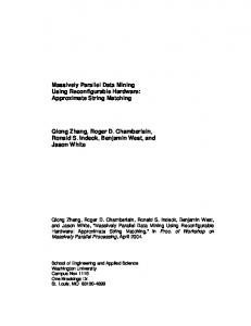
Fig. 1. Linear-Chain factor graph with four hidden nodes Y = {a, b, c, d} (white) and four observed nodes X = {1, 2, 3, 4} (gray). Each factor (black square) represents a clique from the underlying dependency graph of the random variables in V = Y ∪ X.

and the threads to the cores. The GPU is capable to manage substantial more threads than real cores are available, since their computations are used to hide memory latency. To achieve the maximum throughput, there always have to exist some threads which perform computations on the cores while other threads are waiting for their memory requests. Exploiting such fine-granular data-parallelism is normally non-trivial. Designpatterns for parallel algorithms help to get the most out of a GPU. The main pattern is parallel reduction, which is a generic parallelization of functions satisfying the associative property. We used the reduction code by Harris [13], which is known to achieve the maximum throughput, whenever possible, e.g. in any data-parallel summation and maximization. 2.2

Conditional Random Fields

Conditional Random Fields (CRF) is a probabilistic method for labeling and segmenting data [17]. Unlike generative models, which model the joint density p (y, x) over inputs x and labels y, discriminative models, as are CRFs, directly model p (y | x) for a given input sample x. Furthermore, the dependency among the observations is not explicitly represented, which allows the use of rich, overlapping features. For the ease of notation, the probability p(yU ) is a short-cut for p(u = yu , v = yv , w = yw ), where U = {u, v, w} is a set of random variables and yU ∈ Y |U | is a joint realization of them. We consider factor graphs to represent the graphical structure of the CRF. They encode any exponential family probability distribution [29]. A factor graph G = (V, F, E) is bipartite regarding V and F where V contains the variable nodes and F the factor nodes. The nodes in V represent random variables which decompose into the set of observed nodes X and the set of hidden nodes Y (Fig. 1). Although the domains of these variables may be arbitrarily chosen, we consider the domain Y for hidden nodes and X for the observed ones. Let ∆(f ) ˜ ) its observed neighbors. be the set of hidden neighbors of factor node f and ∆(f Each factor node f ∈ F represents a local function f : Y n × X m → R+ (Eq. 1) which measures the score of the hidden neighbors being in state y∆(f ) given the


5

realization x∆(f ˜ ) of the observed neighbors. For instance, the neighborhoods of ˜ )= the factor nodes f, g from Figure 1 are ∆(f ) = {a, b}, ∆(g) = {b} and ∆(f ˜ ∆(g) = {2}. The scores are typically computed as a log-linear combination of a feature vector φ and its corresponding real-valued parameter vector θ. For notational convenience, let the set of hidden nodes be Y = {1, . . . , n}. The features are user-defined binary indicator functions which evaluate to 1 only for a single combination of class label(s) and observed realization. E D . (1) φ y∆(f ) , x∆(f f y∆(f ) | x∆(f ˜ ) ,θ ˜ ) = exp As an implication of the fundamental theorem of random fields [12], the conditional probability mass function (Eq. 2) is given by the normalized product of all local functions. Y p (y | x) = Z(x)−1 f y∆(f ) | x∆(f . (2) ˜ ) f ∈F

Z (x) =

X Y

f y∆(f ) | x∆(f . ˜ )

(3)

y∈Y n f ∈F

The normalization Z(x) is computed as sum of scores for all possible assignments to the hidden nodes. We call a joint hidden node realization y∆(f ) familiar to ˜ ) if there is an instance in the training data where the nodes from xv , v ∈ ∆(f ∆(f ) have the realization y∆(f ) and the observed node v has the realization xv . A realization y∆(f ) or xv is called familiar, if it ever occurs in the training data. To avoid overfitting, weights for unfamiliar realizations are not created during training. In order to train a CRF, the Maximum-Likelihood (ML) method is used. Given a training set T = {(y, x)(i) }1≤i≤N the ML method yields the LogLikelihood (Eq. 4) as the objective function for CRF training. L (θ; T ) =

N X

log p y(i) | x(i) .

(4)

i=1

Common optimization techniques for CRFs like quasi-Newton or stochastic gradient [2] methods rely on the gradient of this objective function to update the model parameters. Equation 5 shows a short-cut writing of the partial derivatives from which the gradient could be computed. The left term is known as the empirical expectation: the number of occurrences of realization y∆(f ) given xv with respect to the training set. Let v be an observed neighbor of factor node f . ∂L (θ; T ) ˜ #f,y ˆ #f,y =E −E . ∆(f ) ,xv ∆(f ) ,xv ∂θf,y∆(f ) ,xv

(5)

The right term represents CRF’s expectation about this number. It is computed by summing the marginal probabilities of the realization y∆(f ) in all training instances that contain the observation xv at observed node v (Eq. 6).

6


N X (i) ˆ #f,y E = 1 p y , x . (i) ,x ∆(f ) v ∆(f ) ˜ ) {xv =x } ∆(f v

(6)

i=1

In this generic notation, every factor node has its own set of parameters. In case of tied parameters, one has to keep in mind that partial derivatives slightly change.

3

Algorithms

In the following code snippets, the scope of data-parallel code, sequential loops and function definitions is indicated by indentation. Using the formal definitions from the previous Section, each gradient-based CRF training consists of the following steps. One iteration of CRF training 1: iterate() 2: computeLocalFunctions() 3: computeMarginalDistribution() 4: computeModelExpectation() 5: computeGradient() 6: updateModelParameters() We use stochastic optimization algorithms which process batches of training instances. Each batch B consists of b instances and the training iterations are performed on any of these batches. We decompose the computation of the local functions (Eq. 1) into independent, parallel summations for each instance in the current batch, each factor as well as each hidden node realization which is familiar to the observations contained in the training instances. The resulting parallel pseudocode is shown in the following listing. Parallel computation of local functions 1: computeLocalFunctions() 2: forall training instances i in current batch 3: forall factor f in F 4: for observed neighbors v from f 5: forall joint realizations y familiar to x[v] 6: score[f][y][i] += weight[f][y][x] Notice that the loop in line 4 was not parallelized in order to omit write conflicts in line 6. Since this is the only loop, the step-complexity amounts to Slf (n) = O(∆˜max ). Here, ∆˜max is the size of the biggest observed neighborhood and ∆max is the size of the biggest hidden neighborhood. As the total number of familiar hidden node realizations is a function of the training set and therefore unknown, we bound it from above with O(|Y|∆max ). The total number of statements,


7

that all threads perform together, is Wlf (n) = O(b|F |∆˜max |Y|∆max ). The dataparallel code indicated by lines 2 and 3 is distributed over a fixed number τB of thread-blocks. Those blocks execute lines 4 to 6 concurrently with τT threads. The optimal values for τB and τT are basically hardware dependent. We used τB = 1024 and τT = 32 in our experiments, but the total runtime differs only slightly for τB ∈ {128, . . . , 2048}. One may examine [21] for technical details on how to derive an optimal value for different hardware. The distribution of computations over thread-blocks for training instances as well as factor nodes results in a very scaleable parallelization at instance- and node-level. This means that for a fixed ∆max , b training instances on a graph with n factor nodes will result in the same number of parallel computations as 1 instance with bn factor nodes. The following algorithms also rely on this principle. In case of local functions, micro-level parallelism is achieved by simply distributing the additions to the threads within the blocks. To compute the marginal probabilities which are needed to obtain the model expectation, LBP is used. The algorithm consits in alternately sending messages from factor to variable nodes and vice versa. Those messages are described below. The parallel computation of messages is distributed to thread-blocks as it was the case for the local functions. In fact, each consecutive pair of forall statements in the following pseudocode is mapped to a fixed number of thread-blocks which yields parallelism at instanceand node-level. The messages are propagated through the graph until the done predicate is satisfied. Our framework allows message specific convergence √ criteria and simple upper bounds for the number of iterations. We choose n, since if the graph contains long paths over factors with weak potentials, distant vertices are approximately independent [14]. This is clearly an approximation, but it delivers nearly the same results as if the true treewidth is used. The pseudocodes of the methods in lines 10, 12, 13 and 14 are not shown, since they resemble the computations of factor messages and hidden messages, respectively. Parallel computation of marginal probabilities with LBP 1: computeMarginalDistributionLBP(){ 2: while not done 3: forall training instances i in batch 4: forall factor f in F 5: computeFactorMessages(i, f) 6: forall training instances i in batch 7: forall hidden node v in V 8: computeHiddenMessages(i, v) 9: forall training instances i in batch 10: computeNormalization(i) 11: forall factor f in F 12: computeFactorBeliefs(i, f) 13: computeMarginals(i, f) 14: forall hidden node v in V 15: computeHiddenBeliefs(i, v)

8


The belief of a factor node f about the joint realization y∆(f ) is computed by multiplying the local function f (y∆(f ) | x) with all incoming messages about yv from all hidden neighbors v ∈ ∆(f ). For hidden nodes v, the belief about label y ˆ is simply the product of all incoming messages of all adjacent factors f ∈ ∆(v). The normalization Z(x) is obtained by summing all beliefs at an arbitrary node. The factor marginals, which are needed to update the model parameters, are computed in line 12 by dividing the beliefs by the normalization. Equitations 7 and 8 are showing the formal definitions of the messages.

mf →v (y | x) =

X

f (y∆(f )−v , v = y | x)

y∈Y |∆(f )−v|

Y

mw→f (yw | x) . (7)

w∈∆(f )−v

By using parallel reduction, the summation in Eq. 7 is divided into partial sums. This yields O(|Y||∆max |) partial factor messages for each core, which are reduced in lines 9 to obtain the final messages. Notice, that unfamiliar realizations do not appear in the training data and hence not have a weight. Thus, only the scores of the familiar realizations have to be multiplied in line 7. The step-complexity is Sf m (n) = O(∆max ) and the work-complexity is Wf m (n) = O(|Y|∆max ∆2max ). Parallel computation of factor messages 1: computeFactorMessages(training instances i, factor f) 2: forall joint realizations y of hidden neighbors from f 3: for hidden neighbor v from f 4: prod := 1 5: for hidden neighbor u not equal v 6: prod *= hiddenMessage[u][f][y[u]][i] 7: if(familiar(y)) prod *= score[f][y][i] 8: FactorMessage[f][v][y[v]][i] += prod 9: reduceFactorMessages() A variable message (Eq. 8) from hidden node v to factor node f about the label y is computed as the product of all incoming factor messages except for the one from f . mv→f (y | x) =

Y

mg→v (y | x) .

(8)

g∈∆(v)−f

The computation of the hidden messages mv→f (y | x) is parallelized by assigning each node from each training instance to a thread-block. by using reduction. This results in a step-complexity of Svm (n) = O(∆ˆ2max ) and an upper bound of Wvm (n) = O(|Y|∆ˆ2max ) for the total number of executed statements, where ∆ˆmax is the biggest neighborhood of all hidden nodes.


9

Parallel computation of hidden messages 1: computeHiddenMessages(training instances i, hidden node v) 2: for neighbor f from v 3: for neighbor g from v not equal f 4: forall single node realization y 5: hiddenMessage[v][f][y][i] *= factorMessage[g][v][y][i] 6: reduceHiddenMessages() Once the marginal probabilities are ready, the model expectation can be computed. All occurrences of familiar observed node realizations xv in the current batch are stored in lists. Those lists are processed iteratively but for all familiar observations in parallel. The marginal probabilities of all joint realizations of hidden nodes which are familiar to the current observation are added to their corresponding expectation. Parallel computation of model expectation 1: computeModelExpectation() 2: forall familiar observed node realization x 3: for occurence (i,f) of x in batch 4: forall familiar to x hidden node realization y 5: expectation[parameterIdx(y,x)] += marginal[y][f][i] Every parameter weights one familiar combination of hidden and observed node realizations. The method parameterIdx is based upon a unique mapping from realizations to natural numbers, which is used to address the expectation array. When the computation has finished, the entries of the gradient-vector can be computed by distributing the computations evenly over all thread in all thread-blocks. The work-complexity is equal to the length of the parameter vector. Parallel computation of the gradient 1: computeGradient() 2: forall parameter p 3: Gradient[p] = -(count[p] - expectation[p]) ˜ i.e. the absolute freThe array count contains the empirical expectation E, quencies of the familiar realizations in the current batch. We store the negative gradient, since we use minimization techniques to maximize the likelihood. To complete a training iteration, we use Stochastic Gradient Descent (SGD) to compute the parameter update. It resembles plain gradient descent for every batch. That is, the η-scaled gradient is substracted from the current parameter vector. Parallel SGD parameter update 1: updateModelParametersSGD() 2: forall parameter p 3: parameter[p] -= eta * gradient[p] The complexities are equal to those of the gradient computation.

10


CRFSGD FB@GPU LBP@GPU FACTORIE F1 -Score 93.73 93.65 93.11 92.74 Precision 93.89 93.83 93.29 92.26 Recall 93.56 93.47 92.94 93.22 Accuracy 96.03 96.00 95.74 95.43 Runtime 296.66 76.42 279.7 808.2 Table 1. Accuracy and runtime on the CoNLL-2000 data set after 10 iterations; runtime in seconds; precision, recall, and F-score in percent; best results in bold; FB@GPU and LBP@GPU are our new algorithms.

4

Evaluation

We use the CoNLL-2000 data set to evaluate our CRF framework. The training set consists of 8936 sentences, each word is annotated with part-of-speech (POS) tags. The task is to label each word with a label indicating whether the word is outside a chunk, starts a chunk, or continues a chunk and the determination of the chunk type. We measure the time for 10 training iterations (including reading the examples) as well as accuracy, precision, recall and F1 -score on a test set of 2012 sentences. The evaluation was run on an AMD 1090T CPU with 8 GiB memory and a NVIDIA C2050 GPU with 3 GiB memory. This evaluation compares our CRF for general factor graphs (LBP@GPU) and our specialized linear-chain CRF inference (FB@GPU) with the sequential CPU algorithms of Leon Bottou’s CRFSGD1 and FACTORIE2 by McCallum et al. For our framework and CRFSGD, the structure of the training data is given by Fig. 1. In fact, our framework uses exactly the same data format (GraphML) which was used to generate Fig. 1. This way, it is possible to load arbitrary graphical models without writing a single line of code. For FACTORIE, their ChainNER3 example was used. We choose words, POS tags, and words in the neighborhood of a given word as observed node realisations, taking into account only those features which occur at least once in the training data. CRFSGD’s learning rate was automatically determined to be η = 5 · 10−2 . We choose ηGP U = 2 · 10−2 and b = 128 for our framework. Table 1 shows the result of the evaluation. While CRFSGD outperforms the other candidates in terms of absolute prediction quality, our specialized FB@GPU inferer attains nearly the same result with ≈ 1/10 of FACTORIE’s runtime. It is worth to say that this kind of inference is deterministic and yields exactly the same result in every run. The general inference approaches perform slightly worth in terms of quality when compared to the specialized variants, yet both are approximations. Nevertheless, our LBP@GPU inference is faster than CRFSGD and FACTORIE. Notice that FACTORIE used the MCMC-sampling for inference, since belief propagation is not supported until now. The binaries and source code of our framework are available for download at http://sfb876.tu-dortmund.de/crfgpu. 1 2

CRFSGD-1.3 is available at http://leon.bottou.org/projects/sgd FACTORIE-0.9.2 is available at http://code.google.com/p/factorie


5

11

Conclusion and Future Work

For general graphical structures we could show, that training CRFs on GPUs outperforms one of the most sophisticated graphical modelling frameworks as well as a specialized linear-chain CRF implementation. Even though it is known that the here applied flooding message schedule performs unnecessary message computations, our algorithm delivers a reasonable runtime. It is planned to add more sophisticated message schedules like ResidualSplash to our framework. Also the MCMC-sampling which is used by FACTORIE is an extension we consider. The graphical model from our evaluation contains only 78 nodes, hence we will present results on larger models in future. First experiments on models with several thousand nodes showed, that our node-level parallelization scales very good, as expected. Our parallel forward-backward algorithm is clearly the fastest linear-chain CRF trainer around. This also shows, that the comparsion of general inference frameworks with specialized, fixed-graph algorithms will always yield worse performance for the general variants in terms of runtime. Acknowledgments. This work has been supported by the DFG, Collaborative Research Center SFB876, project A1.

References 1. Athanasopoulos, A., Dimou, A., Mezaris, V., Kompatsiaris, I.: GPU acceleration for support vector machines. In: Procs. 12th Inter. Workshop on Image Analysis for Multimedia Interactive Services (WIAMIS 2011), Delft, Netherlands (2011) 2. Bottou, L.: Large-scale machine learning with stochastic gradient descent. In: Lechevallier, Y., Saporta, G. (eds.) Procs. of the 19th International Conference on Computational Statistics. pp. 177–187. Springer, Paris, France (2010) 3. Bottou, L., LeCun, Y.: On-line learning for very large datasets. Applied Stochastic Models in Business and Industry 21(2), 137–151 (2005) 4. Catanzaro, B., Sundaram, N., Keutzer, K.: Fast support vector machine training and classification on graphics processors. In: Procs. of the 25th international conference on Machine learning. pp. 104–111. ACM (2008) 5. Chao-Chung, C., Chung-Te, L., Chia-Kai, L., Yen-Chieh, L., Liang-Gee, C.: Architecture design of stereo matching using belief propagation, pp. 4109–4112 (2010) 6. Craven, M., DiPasquo, D., Freitag, D., McCallum, A., Mitchell, T., Nigam, K., Slattery, S.: Learning to extract symbolic knowledge from the world wide web. In: Procs. of the 15th nat. conf. on Arti. intell. pp. 509–516. AAAI ’98/IAAI ’98, American Ass. for Arti. Intell., Menlo Park, CA, USA (1998) 7. Fang, W., Lu, M., Xiao, X., He, B., Luo, Q.: Frequent itemset mining on graphics processors. In: DaMoN ’09: Procs. of the Fifth International Workshop on Data Management on New Hardware. pp. 34–42. ACM, New York, NY, USA (2009) 8. Gonzalez, J.E., Low, Y., Guestrin, C.: Residual splash for optimally parallelizing belief propagation. In: Arti. Intell. and Stat. (AISTATS. pp. 177–184 (2009) 9. Gonzalez, J.E., Low, Y., Guestrin, C., O’Hallaron, D.: Distributed parallel inference on large factor graphs. In: Procs. of the 25th Conf. on Uncertainty in Arti. Intell. pp. 203–212. UAI ’09, AUAI Press, Arlington, Virginia, USA (2009)

12


10. Grauer-Gray, S., Kambhamettu, C.: Hierarchical belief propagation to reduce search space using cuda for stereo and motion estimation. In: Applications of Computer Vision (WACV), 2009 Workshop on. pp. 1–8 (2009) 11. Grauer-Gray, S., Kambhamettu, C., Palaniappan, K.: Gpu implementation of belief propagation using cuda for cloud tracking and reconstruction. In: Pattern Recognition in Remote Sensing (PRRS 2008), 2008 IAPR Workshop on. pp. 1–4 (2008) 12. Hammersley, J.M., Clifford, P.: Markov fields on finite graphs and lattices (1971) 13. Harris, M.: Optimizing Parallel Reduction in CUDA. NVIDIA Corporation (2008) 14. Ihler, A.T., Fischer III, J.W., Willsky, A.S.: Loopy belief propagation: Convergence and effects of message errors. J. Mach. Learn. Res. 6, 905–936 (December 2005) 15. J´ aJ´ a, J.: An introduction to parallel algorithms. Addison Wesley Longman Publishing Co., Inc., Redwood City, CA, USA (1992) 16. Kschischang, F.R., Frey, B.J., Loeliger, H.A.: Factor graphs and the sum-product algorithm. IEEE Transactions on Information Theory 47(2), 498–519 (2001) 17. Lafferty, J., McCallum, A., Pereira, F.: Conditional random fields: Probabilistic models for segmenting and labeling sequence data. Procs. 18th International Conf. on Machine Learning pp. 282–289 (2001) 18. Lai, Y.C., Cheng, C.C., Liang, C.K., Chen, L.G.: Efficient message reduction algorithm for stereo matching using belief propagation. Img.Pr. 1(2), 2977–2980 (2010) 19. Low, Y., Gonzalez, J., Kyrola, A., Bickson, D., Guestrin, C., Hellerstein, J.M.: Graphlab: A new parallel framework for machine learning. In: Conference on Uncertainty in Arti. Intell. (UAI). Catalina Island, California (July 2010) 20. McCallum, A., Schultz, K., Singh, S.: Factorie: Probabilistic programming via imperatively defined factor graphs. In: Neural Infor. Proc. Sys. (NIPS) (2009) 21. NVIDIA Corporation: CUDA Programming Guide 4.0 (June 2011) 22. Pearl, J.: Probabilistic reasoning in intelligent systems: networks of plausible inference. Morgan Kaufmann Publishers Inc., San Francisco, CA, USA (1988) 23. Phan, X.H., Nguyen, L.M., Inoguchi, Y., Horiguchi, S.: High-performance training of conditional random fields for large-scale applications of labeling sequence data. IEICE - Trans. Inf. Syst. E90-D, 13–21 (January 2007) 24. Roth, D.: On the hardness of approximate reasoning. Arti.Inte. 82, 273–302 (1996) 25. Saxena, A., Chung, S.H., Ng, A.Y.: 3-d depth reconstruction from a single still image. International Journal of Computer Vision (IJCV 76, 53–69 (2007) 26. Settles, B.: Biomedical named entity recognition using conditional random fields and rich feature sets. In: Procs. of the International Joint Workshop on Natural Language Processing in Biomedicine and its Applications. pp. 104–107. JNLPBA ’04, Ass. for Comp. Linguistics, Stroudsburg, PA, USA (2004) 27. Sun, J., Zheng, N.N., Member, S.: Stereo matching using belief propagation. IEEE Transactions on Pattern Analysis and Machine Intell. 25(7), 787–800 (2003) 28. Vishwanathan, S.V.N., Schraudolph, N.N., Schmidt, M.W., Murphy, K.P.: Accelerated training of conditional random fields with stochastic gradient methods. In: ICML ’06: Procs. of the 23rd international conference on Machine learning. pp. 969–976. ACM, New York, NY, USA (2006) 29. Wick, M., McCallum, A., Miklau, G.: Scalable probabilistic databases with factor graphs and MCMC. Procs. VLDB Endow. 3, 794–804 (September 2010) 30. Xiao, H.: Towards Parallel and Distributed Computing in Large-Scale Data Mining: A Survey. Tech. rep., Technical University of Munich, Germany (2010) 31. Yanover, C., Schueler-Furman, O., Weiss, Y.: Minimizing and learning energy functions for side-chain prediction. In: Procs. of the 11th annual int. conf. on Research in comp. molecular biology. pp. 381–395. RECOMB’07, Springer, Berlin, Heidelberg (2007)