The implementation of a complete backtrack search parallel algorithm de- scribed in this document incorporates most of the state-of-the-art sequential.
Tel-Aviv University Raymond and Beverly Sackler Faculty of Exact Sciences The School of Computer Science
Parallel Multithreaded Satisfiability Solver: Design and Implementation
A thesis submitted in partial fulfillment of the requirements for the degree of Master of Science
by
Yulik Feldman
The research work in this thesis has been carried out under the supervision of Prof. Nachum Dershowitz
January 2005
Abstract This thesis describes the design and implementation of a highly optimized, multithreaded algorithm for the propositional satisfiability problem. The algorithm is based on the Davis-Logemann-Loveland sequential algorithm, but includes many of the optimization techniques introduced in recent years. The document provides experimental results for the execution of the parallel algorithm on a variety of multiprocessor machines with shared memory architecture. In particular, the overwhelming effect of parallel execution on the performance of processor cache is studied.
Contents 1 Introduction
3
2 The SAT problem and basic terminology
5
3 Sequential SAT algorithms
8
3.1
DLL algorithm . . . . . . . . . . . . . . . . . . . . . . . . . . . .
8
3.1.1
Backtrack search . . . . . . . . . . . . . . . . . . . . . . .
8
3.1.2
Boolean constraint propagation (BCP) . . . . . . . . . . .
10
Conflict-driven learning . . . . . . . . . . . . . . . . . . . . . . .
14
3.2.1
Implication graph
. . . . . . . . . . . . . . . . . . . . . .
15
3.2.2
Conflict clauses . . . . . . . . . . . . . . . . . . . . . . . .
17
3.2.3
Non-chronological backtracking . . . . . . . . . . . . . . .
19
3.2.4
Conflict clause deletion . . . . . . . . . . . . . . . . . . .
19
3.3
Branching heuristics . . . . . . . . . . . . . . . . . . . . . . . . .
19
3.4
Restarts . . . . . . . . . . . . . . . . . . . . . . . . . . . . . . . .
21
3.2
4 Parallel SAT algorithms
22
4.1
Search space partitioning . . . . . . . . . . . . . . . . . . . . . .
22
4.2
Task scheduling . . . . . . . . . . . . . . . . . . . . . . . . . . . .
24
4.3
Conflict clause exchange . . . . . . . . . . . . . . . . . . . . . . .
26
4.4
Thread synchronization overhead . . . . . . . . . . . . . . . . . .
28
5 Solver implementation 5.1
30
Data-oriented classes . . . . . . . . . . . . . . . . . . . . . . . . .
31
5.1.1
CAssignment . . . . . . . . . . . . . . . . . . . . . . . . .
31
5.1.2
CClause . . . . . . . . . . . . . . . . . . . . . . . . . . . .
31
5.1.3
CConfiguration . . . . . . . . . . . . . . . . . . . . . . . .
32
1
5.2
5.3
5.1.4
CImplication . . . . . . . . . . . . . . . . . . . . . . . . .
33
5.1.5
CLemmaContainer . . . . . . . . . . . . . . . . . . . . . .
34
5.1.6
CLiteral . . . . . . . . . . . . . . . . . . . . . . . . . . . .
34
5.1.7
CStatistics . . . . . . . . . . . . . . . . . . . . . . . . . .
34
5.1.8
CTask . . . . . . . . . . . . . . . . . . . . . . . . . . . . .
36
5.1.9
CVariable . . . . . . . . . . . . . . . . . . . . . . . . . . .
37
Algorithm-oriented classes . . . . . . . . . . . . . . . . . . . . . .
39
5.2.1
CClauseBuilder . . . . . . . . . . . . . . . . . . . . . . . .
39
5.2.2
CConflictAnalysis . . . . . . . . . . . . . . . . . . . . . .
39
5.2.3
CDecisionStrategy . . . . . . . . . . . . . . . . . . . . . .
42
5.2.4
CParser . . . . . . . . . . . . . . . . . . . . . . . . . . . .
44
5.2.5
CSolver . . . . . . . . . . . . . . . . . . . . . . . . . . . .
44
5.2.6
CTaskList . . . . . . . . . . . . . . . . . . . . . . . . . . .
45
5.2.7
CThread
. . . . . . . . . . . . . . . . . . . . . . . . . . .
47
Other classes and algorithms . . . . . . . . . . . . . . . . . . . .
51
5.3.1
CIndexWeightPairLess . . . . . . . . . . . . . . . . . . . .
51
5.3.2
CTaskLess . . . . . . . . . . . . . . . . . . . . . . . . . . .
51
5.3.3
CThreadId . . . . . . . . . . . . . . . . . . . . . . . . . .
51
5.3.4
main() function . . . . . . . . . . . . . . . . . . . . . . . .
51
6 Testing environment
52
7 Experimental performance results
56
8 Related work
64
9 Conclusion
66
2
Chapter 1
Introduction This thesis describes the design and implementation of a highly optimized, parallel multithreaded algorithm for solving the propositional satisfiability problem (SAT). SAT is a fundamental problem in the theory of computation, one that has been studied extensively for more than four decades, ever since the introduction of the first algorithm for its solution in 1960 [7]. Eleven years later it became the first problem proven to be NP-complete, in a famous paper by Cook [5]. Nowadays, the problem evidences great practical importance in a wide range of disciplines, including hardware verification [30], artificial intelligence [18], computer vision [4] and others. Indeed, one survey of satisfiability [9] contains over 200 references to applications. In spite of its computational complexity, there is strong demand in industry for high-performance SAT-solving algorithms. Over the years, many different approaches and optimizations have been developed to tackle the problem more efficiently. Algorithms have evolved gradually by extending existing methods with new, more powerful, optimizations. Current research on propositional satisfiability is focused on two classes of SAT solving methods: complete algorithms and incomplete procedures. Complete methods, mostly represented by backtrack search algorithms, identify both satisfiable and unsatisfiable problems, and show reasonably good performance on both types. Incomplete methods, mostly represented by variations of local search procedures, perform much faster on satisfiable problems, but incur the price of not always being able to demonstrate unsatisfiability. The fact that backtrack search algorithms are able
3
to cope with unsatisfiable problems usually makes them the preferred choice in domains where proofs of unsatisfiability are required. The implementation of a complete backtrack search parallel algorithm described in this document incorporates most of the state-of-the-art sequential technologies introduced in recent years. The emphasis has been on providing an efficient portable implementation that would work on any typical multiprocessor workstation in an industrial environment and improve runtime, as compared with the core sequential algorithms, by distributing the workload over several processors on one machine. To make sure the implementation is efficient and that low-level implementation details are properly understood, the implementation of the solver was not based on existing publicly available source code of other solvers, but instead was designed and coded from scratch. The implementation was carefully crafted to enable a direct comparison of its behavior with existing sequential algorithms. After the implementation of the algorithm was completed, its behavior in different real-life environments was measured. In particular, the effect of concurrent execution of multiple threads on the behavior of platform architecture primitives, such as processor cache, bus utilization and resource allocation, was investigated. The main contribution of this work is that it shows the general disadvantageousness of parallel execution of a backtrack search algorithm on a multiprocessor workstation, due to increased cache misses. The remainder of this document is organized as follows: the next chapter describes the SAT problem and basic terminology. Chapter 3 gives an overview of the state-of-the-art sequential algorithms used in the implementation of the solver, while Chapter 4 describes the methods used to parallelize these algorithms. Chapter 5 shows implementation details of the solver, and Chapter 6 gives an overview of tools and methods used to test the implementation. Chapter 7 reports on the results of experimental runs of the solver in various configurations. Chapter 8 describes related work in the area of parallel SAT solving, and is followed by a brief conclusion. A paper on this work was presented at 3rd International Workshop on Parallel and Distributed Methods in Verification (PDMC 2004) [1] and published in [10].
4
Chapter 2
The SAT problem and basic terminology The propositional satisfiability problem can be formulated easily in one sentence: given a boolean formula, determine whether an assignment of boolean truth values to the propositional variables in the formula exists, such that the formula evaluates to true. If such an assignment exists, the formula is said to be satisfiable; if no such assignment exists, it is unsatisfiable. This chapter describes the basic terminology used in discussions of satisfiability problem. More advanced terminology, used in the context of specific SAT solving algorithms, is given in the next chapter. Although there are many ways to represent a boolean formula, conjunctive normal form (CNF) is most frequently used for this purpose. In general, it is not a limitation to use CNF for the representation of formulas, since any boolean formula can be transformed to an equivalently satisfiable formula in CNF (with extra variables) in polynomial time [26]. In CNF, the variables of the formula appear in literals, which are either a lone variable (x) or the negation of a variable (¯ x). Literals are grouped into clauses, which represent a disjunction (logical or ) of the literals they contain. A single literal can appear in any number of clauses. The conjunction (logical and ) of all clauses represents a formula. For example, the CNF formula (x1 ∨ x ¯2 ) ∧ (¯ x3 ) ∧ (x1 ∨ x3 ) contains three clauses: x1 ∨ x ¯2 , x ¯3 and x1 ∨ x3 . Two literals in these clauses are positive (x1 , x3 ) and two are negative (¯ x2 , x ¯3 ). Note that for a variable assignment to
5
satisfy a CNF formula, it must satisfy each of its clauses. For example, if x 1 is true and x3 is false, then all three clauses are satisfied, regardless of the value of x2 . A boolean variable can be assigned one of two boolean truth values: false or true. The false value is sometimes referred as the value zero (0), while the true value is sometimes referred to as one (1). If a variable is assigned a truth value, it is said that it is an assigned variable. If a variable is not assigned a truth value, its value is undetermined, or irrelevant, and it is said that the variable is unassigned variable. Similarly, literals are also said to be assigned or unassigned. When a variable is assigned a specific value v, the positive literals based on this variable are assigned the value v and the negative literals based on this variable are assigned the opposite value. Given an assignment to all formula variables, the value of each clause and the value of the whole formula are evaluated according to the semantics of logical operations. If the clause evaluates to true, it is said that the assignment satisfies the clause, or, alternatively, the clause is satisfied. If the clause evaluates to false, it is said that the assignment does not satisfy the clause, or, alternatively, the clause is unsatisfied. If all formula clauses evaluate to true, the formula also evaluates to true and is said to be satisfied. If at least one clause evaluates to false, the formula evaluates to false and is said to be unsatisfied. As mentioned above, if an assignment to formula variables exists such that the formula is satisfied, the formula is said to be satisfiable and such an assignment is called a satisfying assignment. On the other hand, if no such assignment exists, the formula is unsatisfiable. All possible assignments to variables of such a formula are unsatisfying. Existence of a satisfying assignment for a given formula is referred to as satisfiability of the formula. If a variable assignment assigns a value to all formula variables, it is called a full assignment. For a formula with n variables, there are 2n possible full assignments. If only some of the formula variables are assigned, such an assignment is called partial. Note that if the same literal appears more than once in a single clause, the additional instances of the literal may be easily removed from the clause without affecting the satisfiability of the formula. In the following discussions, it is assumed that at most one instance of each literal is found in each clause, based on the presumption that redundant literal instances have been removed
6
during early stages of the SAT-solving algorithm. Another easily detectable redundancy is the case when both positive and negative literals of the same variable are present in the same clause. In such a case, the clause and the formula can not be satisfied by any assignment. It is assumed that such cases are also detected in early stages of the algorithm and therefore do not have to be taken care of at later stages.
7
Chapter 3
Sequential SAT algorithms The sequential SAT solving algorithm used in the implementation of the parallel SAT solver is based on the commonly used Davis-Logemann-Loveland algorithm (DLL) [6]. The following sections describe the original DLL algorithm and a number of optimization techniques that can enhance the original algorithm to achieve better results. All the techniques shown in this chapter were implemented in the parallel SAT solver described in this document.
3.1
DLL algorithm
The Davis-Logemann-Loveland algorithm is a backtrack search SAT-solving algorithm extended with an optimization technique called boolean constraint propagation. The following sections describe the principles of a backtrack search SAT solving algorithm and the boolean constraint propagation optimization technique.
3.1.1
Backtrack search
The backtrack search algorithm performs a methodical search of variable assignments, trying to satisfy the formula. To build the variable assignments, the algorithm chooses variables in a certain order and incrementally assigns a value to each variable. As long as the resulting partial variable assignment does not falsify the formula, the algorithm continues to choose variables and assign a value to the chosen variables. If the resulting partial variable assignment falsi-
8
fies the formula, the algorithm assigns an opposite value to the last variable it chose and checks whether the resulting assignment still falsifies the formula. If the formula becomes satisfied, the algorithm proceeds with assigning more variables. If the formula is falsified independently of the value of the last assigned variable, the algorithm backtracks to the previous variable and assigns it an opposite value. The algorithm continues the search in similar fashion, assigning, reassigning and unassigning variable values until either all variables are assigned and the formula is satisfied or until all possible variable assignments are covered and no satisfiable assignment is found. Note that the algorithm does not explicitly visit all 2n assignments, since it backtracks once a partial unsatisfying assignment is found. Still, the complexity of the algorithm is exponential. The above algorithm can be also described as a depth-first-search (DFS) algorithm on a binary tree of partial variable assignments. Each node in that tree represents a partial variable assignment. Each node has two children nodes, representing an extension of the partial variable assignment of the node with assignment to another variable, assigning the false value for the first children node and the true value for the second. The depth of the binary tree equals the number of variables in the formula. The leaves of the tree represent the full variable assignments. The number of leaves is 2n , corresponding to the total number of full variable assignments. The DLL algorithm can be seen as a DFS traversal of that tree, in which the algorithm backtracks as soon as it reaches a node representing an unsatisfying partial assignment. The algorithm ends when it reaches a node representing satisfying partial or full assignment (in which case it reports satisfiability of the formula), or when the whole tree is traversed (in which case it reports unsatisfiability of the formula). The tree of partial variable assignments is commonly called the search tree. The traversal of the search tree combined with the backtracks is commonly called backtrack search. Figure 3.1 shows an example of a search tree for the formula (x1 ∨ x2 ∨ x ¯3 ) ∧ (¯ x3 ∨ x4 ) ∧ (x2 ∨ x3 ). Note that each level in the search tree in Figure 3.1 corresponds to an assignment to a particular variable, while the variables are ordered from x1 to x4 from the top of the tree to the bottom. Such a fixed order is not compulsory and may change according to algorithm heuristics, which will be described later. Figure 3.2 shows the steps taken by basic backtrack search algorithm while traversing the tree shown in Figure 3.1.
9
X X1 = 0
X1 = 1
X
X
X2 = 0
X2 = 1
X X 3 = 0 X3 = 1 0
0
0
0
0
X2 = 0 X
X
X3 = 0 X3 = 1
X3 = 0 X3 = 1
1
0
1
X
1
0
X
0
1
0
X2 = 1
X3 = 0 X 3 = 1
X
0
0
1
1
1
X
1
0
1
Figure 3.1: Search tree for the formula (x1 ∨ x2 ∨ x ¯3 ) ∧ (¯ x3 ∨ x4 ) ∧ (x2 ∨ x3 )
3.1.2
Boolean constraint propagation (BCP)
The original Davis-Logemann-Loveland algorithm used an optimization technique called unit propagation, or boolean constraint propagation (BCP ). If the current partial variable assignment causes all but one literal of some clause to be assigned the false value, the remaining literal has to be assigned true in order to not falsify the clause and the formula. Such a literal is called a unit literal, and such a clause is called a unit clause. If a unit clause is found, the algorithm chooses the variable of the unit literal as the next variable to assign a value to, and assigns it a value that makes the unit literal evaluate to true. If more than one unit clause is found, the algorithm collects all unit literals and uses them in the subsequent variable assignments. Such variable assignments are called implications. Note that more clauses may become unit clauses as a result of evaluating the initial implications. The process of finding unit clauses and creating the implications continues until an implication assigning an opposite value to the already assigned variable is found or until no more unit clauses are found. This process is called boolean constraint propagation. To distinguish between the variables assigned as a result of boolean constraint propagation and the variables assigned by the main DLL algorithm, the variables assigned as a result of boolean constraint propagation are called implication variables, and the other variables are called decision variables.
10
1. Choose first variable (x1 ) and assign it 0. 2. Current partial assignment: x1 = 0. This partial assignment evaluates to unknown (the value of the formula can not be determined). Choose next variable (x2 ) and assign it 0. 3. Current partial assignment: x1 = 0, x2 = 0. This partial assignment evaluates to unknown. Choose next variable (x3 ) and assign it 0. 4. Current partial assignment: x1 = 0, x2 = 0, x3 = 0. This partial assignment evaluates to false, since it makes the third clause evaluate to false. Since the last assigned variable (x3 ) was not yet assigned both values, assign it the opposite value (1). 5. Current partial assignment: x1 = 0, x2 = 0, x3 = 1. This partial assignment evaluates to false, since it makes the first clause evaluate to false. Since the last assigned variable was already assigned both values, backtrack. 6. Current partial assignment: x1 = 0, x2 = 0. This partial assignment evaluates to unknown. However, it is now known that when this assignment is extended with variable x3 it evaluates to false, independently of the value of that variable. Since the last assigned variable (x2 ) was not yet assigned both values, assign it the opposite value (1). 7. Current partial assignment: x1 = 0, x2 = 1. This partial assignment evaluates to unknown. Choose next variable (x3 ) and assign it 0. 8. Current partial assignment: x1 = 0, x2 = 1, x3 = 0. This partial assignment evaluates to true, since it makes all clauses evaluate to true. Finish the algorithm and report that the formula is satisfiable by the current partial assignment.
Figure 3.2: Steps taken by basic backtrack search algorithm while traversing the tree shown in Figure 3.1
11
The situation in which an implication assigns an opposite value to the already assigned variable is called a conflict. If a conflict is found, the DLL algorithm assigns the opposite value to the last assigned decision variable or, alternatively, backtracks, if that variable was already assigned both values. If no more unit clauses are found, the DLL algorithm continues with choosing the next decision variable. Each assignment to a decision variable is said to increase the decision level of the algorithm. Correspondingly, each unassignment of a decision variable (backtracking) is said to decrease the decision level. An assignment to an implication variable does not change the decision level. Each variable, either a decision variable or an implication variable, has a decision level associated with it. This is the decision level of the algorithm on which the variable has been assigned a value. Therefore, at every given point of algorithm execution, a single decision variable and zero or more implication variables are associated with each decision level. Figure 3.3 shows the steps taken by the backtrack search algorithm with boolean constraint propagation (basic DLL) on formula (x2 ∨ x ¯3 ) ∧ (x2 ∨ x3 ∨ x ¯4 ) ∧ (x1 ∨ x4 ). The boolean constraint propagation algorithm should be able to detect unit clauses and the clauses falsified by the current variable assignments in a very efficient way. A number of techniques for doing this have been proposed over the years. One technique is the ”two watching literals” scheme proposed in [23]. With this technique, two arbitrary literals not assigned false in each clause are marked as special watching literals. The watching literals are associated with the variables on which the literals are based. When a variable is assigned a value, the clauses that have the watching literals based on this variable are checked. The clauses that do not have watching literals based on this variable can not become unit clauses, since at least two other literals of the clauses, which are the watching literals based on other variables, are not assigned false. These clauses may be safely ignored in the process of searching for implied unit clauses. The clauses that have the watching literals based on the assigned variable can potentially become unit clauses and therefore are checked. For each such clause, if the clause did not become a unit clause as a result of variable assignment, another clause literal not currently assigned false is marked as a watching literal and the algorithm continues.
12
1. Choose first decision variable (x1 ) and assign it 0. 2. Current partial assignment: x1 = 0. Decision level is 1. This partial assignment evaluates to unknown. The third clause (x1 ∨ x4 ) is a unit clause, since all its literals but one (x4 ) are assigned 0. The literal x4 is the unit literal. Create implication x4 = 1. 3. Current partial assignment: x1 = 0, x4 = 1. Decision level is 1. This partial assignment evaluates to unknown. No more clauses become unit clauses. Continue regular backtrack search by choosing the next decision variable (x2 ) and assigning it the value 0. 4. Current partial assignment: x1 = 0, x2 = 0, x4 = 1. Decision level is 2. This partial assignment evaluates to unknown. The first clause becomes a unit clause. The literal x3 is the unit literal. Create implication x3 = 0. The second clause also becomes a unit clause as a result of the original assignment. The literal x3 is the unit literal in this clause as well. However, the implication created for this clause is x3 = 1. Since the opposite values are being assigned to the same variable, a conflict is created. To resolve the conflict, assign the opposite value (1) to the last decision variable (x2 ). 5. Current partial assignment: x1 = 0, x2 = 1, x4 = 1. Decision level is 2. This partial assignment evaluates to true, since it makes all clauses evaluate to true. Finish the algorithm and report that the formula is satisfiable by the current partial assignment.
Figure 3.3: The steps taken by backtrack search algorithm with boolean constraint propagation (basic DLL) on formula (x2 ∨ x ¯3 ) ∧ (x2 ∨ x3 ∨ x ¯4 ) ∧ (x1 ∨ x4 )
13
The two watching literals scheme is very efficient, since the clauses that do not have watching literals based on the recently assigned variable do not need to be checked for becoming a unit clause.
3.2
Conflict-driven learning
In 1996, Marques-Silva and Sakallah proposed an important optimization technique for the core DLL algorithm, called conflict-driven learning [20]. Conflictdriven learning is a combination of conflict analysis, conflict learning, and a conflict-directed backjumping, also called non-chronological backtracking. The conflict analysis is invoked when boolean constraint propagation finds a conflict. The purpose of conflict analysis is to find the reasons that caused the conflict. The algorithm does so by building and analyzing a data structure called the implication graph. The implication graph is described in Section 3.2.1. Once the conflict analysis builds the implication graph, it analyzes the graph and builds one or more special formula clauses that record the reasons for the conflict in a form consistent with the original formula clauses. These clauses are called conflict clauses. Section 3.2.2 describes how the conflict clauses are built. Once the conflict clauses are built, the algorithm appends them to the formula, making the information in the clauses available for future search. The process of appending the conflict clauses to the formula is called conflict learning. It helps the core DLL algorithm avoid entering search paths that lead to the previously found conflicts. In addition to building the conflict clauses, the ability of conflict analysis to find the exact reasons for the conflict enables it to find the minimal decision level whose decision unavoidably leads to the current conflict. This in turn makes it possible to implement non-chronological backtracking, which allows the DLL algorithm to backtrack more than one decision level at once. Non-chronological backtracking is described in Section 3.2.3. Conflict-driven learning is one of the most important optimization techniques for the core DLL algorithm. Its introduction and subsequent improvements brought orders of magnitude improvement in the average performance of the algorithm.
14
x4 (3)
x 6 (1)
x12 (5)
x1 (5 ) x2 ( 5)
x11 (5 )
x17 (1)
x8 ( 2)
x 3 (5 ) x18 ( 5 )
x10 ( 5) Decision variable
Conflicting variable
x16 ( 5) x13 ( 2 )
x5 ( 5) x19 ( 3 )
x18 ( 5 )
Figure 3.4: An example of an implication graph
3.2.1
Implication graph
The implication graph is a graph whose nodes represent variable assignments and whose edges represent those unit clauses that implied the variable assignments. The graph is built in the first stage of the conflict analysis algorithm. Since the conflict analysis algorithm is invoked only when a conflict is found, the implication graph always contain a variable assigned two opposite values. The variable that is assigned two opposite values is called a conflicting variable and is represented by two complementary nodes in the implication graph. Figure 3.4 shows an example of an implication graph. The labels on graph nodes denote the variable assignments the nodes represent. The labels specify the variable being assigned, while positive literals of the variable represent assignments of 1 and negative literals represent assignments of 0. The number in parentheses represents the decision level associated with each assignment. The implication graph in Figure 3.4 shows the implications of an assignment to the decision variable x11 on decision level 5 (shown on the left). The graph shows that as a result of this assignment the variable x 18 becomes conflicting. The white nodes represent the assignments made on the same decision level as the assignment to the decision variable (5). The black nodes represent the assignments made on lower decision levels. While there may ex15
ist more assignments made on lower decision levels than the graph shows, only those assignments that are directly connected to the while nodes are shown. The other assignments made on lower decision levels do not participate in the conflict analysis. The edges of the graph are built according to the unit clauses that were used to create the implications shown in the graph. For example, the node x16 (5) represents the assignment to the unit literal of the unit clause (¯ x11 ∨ x13 ∨ x16 ). According to the graph, the variable x16 has been assigned 0 on decision level 2. The variable x11 has been assigned 1 on decision level 5. As a result the clause became a unit clause, with x16 being a unit literal. In order to not falsify the clause and the formula, an implication x16 = 1 has been created on level 5. The edges (x11 (5) → x16 (5)) and (¯ x13 (2) → x16 (5)) in the implication graph represent this implication. The other edges are built in a similar way. Given a graph node, the nodes that are directly connected to it through the incoming edges of that node are called the antecedent nodes of the node (or, alternatively, antecedent vertices). The nodes x11 (5) and x ¯13 (2) are antecedent nodes of the node x16 (5). The unit clause that implies the edges between the node and its antecedent nodes is called the antecedent clause. The clause (¯ x 11 ∨ x13 ∨ x16 ) is the antecedent clause of the node x16 (5) in this example. Note that the node representing an assignment to the decision variable does not have incoming edges and, correspondingly, the antecedent nodes and the antecedent clause. In an implication graph, node x is said to dominate node y if any path from the decision variable to node y needs to go through node x. A unique implication point (UIP ) is a node at the current decision level that dominates both nodes corresponding to the conflicting variable. In the graph in Figure 3.4, node x ¯10 (5) dominates both nodes x18 (5) and x ¯18 (5); therefore, it is a UIP. The decision variable is always a UIP. Note that there may be more than one UIP for a certain conflict. In the example, there are three UIPs, namely, x11 (5), x ¯2 (5) and x ¯10 (5). Intuitively, UIPs represent the reason that implies the conflict at the current decision level. The UIPs are ordered starting from the conflict. In the example, x ¯10 (5) is the first UIP, x ¯2 (5) is the second UIP and x11 (5) is the last UIP.
16
x 4 ( 3)
x 6 (1)
x12 (5)
x1 ( 5 ) x 2 ( 5)
x11 (5 )
x17 (1)
x8 ( 2)
x 3 (5 ) x18 ( 5 )
x10 ( 5) Decision variable
Conflicting variable
x16 ( 5) x13 ( 2 )
x5 ( 5) x19 ( 3 )
x18 ( 5 )
Cut 1 Cut 2 Cut 3
Figure 3.5: Examples of implication graph cuts
3.2.2
Conflict clauses
Conflict clauses are generated by a bipartition of the implication graph. The partition has all the decision variables on one side (called reason side), and the conflicting variable on the other side (the conflict side). All nodes on the reason side that have at least one edge to the conflict side comprise the reason for the conflict. Such a bipartition is called a cut. Different cuts correspond to different learning schemes. Figure 3.5 shows several examples of implication graph cuts. Cut 1 on Figure 3.5 represents the cut nearest to the pair of conflict variable nodes. Cut 2 represents the cut that separates the conflicting variable from the first UIP node (¯ x10 (5)), such that all nodes implied by the first UIP node appear on the conflict side of the cut. Cut 3 represents the cut nearest the decision variable. It is also the cut that separates the conflicting variable from the last UIP node, which is the node of the decision variable. These cuts are only several examples of legal cuts of the given implication graph. There exist more cuts that legally bipartition this graph. Each cut may be represented as a disjunction of negations of literals corresponding to the source nodes of edges that cross the cut. These disjunctions of literals are called conflict clauses. The conflict clause corresponding to Cut 1 17
is (x17 ∨ x ¯1 ∨ x ¯ 3 ∨ x5 ∨ x ¯19 ), to Cut 2 is (x17 ∨ x ¯8 ∨ x10 ∨ x ¯19 ) and to Cut 3 is (x17 ∨ x ¯8 ∨ x ¯ 4 ∨ x6 ∨ x ¯11 ∨ x13 ∨ x ¯19 ). The conflict clauses are clauses that do not exist in the original formula, but may be safely added to it, as they do not change the satisfiability of the formula. It may be shown that the conflict clauses are generated according to the operation called resolution, in which the generated clauses are redundant with respect to the original clauses [35]. There exist different heuristics that generate conflict clauses according to different cuts of the implication graph. The heuristics differ by the size of generated conflict clauses, the average distance of the cuts from the conflicting variable, the correspondence of the cuts to the UIPs of the graph, the number of cuts being taken into account and other characteristics. Some heuristics limit the cuts to the portion of the graph corresponding to the current decision level, while others extend the cuts into the nodes corresponding to lower decision levels. Many such heuristics are analyzed and compared in [34]. The authors empirically show that the heuristic that usually outperforms the others is the one called the first UIP learning scheme. This heuristic corresponds to the cut where the conflict side includes all nodes implied by the first UIP, like Cut 2 in Figure 3.5. The heuristics based on the UIPs are important since they have the property that once the conflict is resolved, as shown in the following section, there exists a single variable whose currently assigned value should be flipped to take the search to a new subspace. The conflict clauses that have this property are called the asserting clauses. The variable whose currently assigned value should be flipped is called the asserting variable. It is always desirable for a conflict clause to be an asserting clause, since it allows a quick decision how to continue the search after resolving the conflict. Many modern implementations of the DLL algorithm use the first UIP learning scheme in their conflict-driven learning algorithms. The conflict clauses contribute to the performance of the DLL algorithm by carrying information on what partial assignments lead to conflicts. When the DLL algorithm encounters similar partial assignments again, the corresponding conflict clause becomes a unit clause, and BCP prevents the algorithm from exploring the implications of the assignments by assigning the non-conflicting value to the unit literal of the clause.
18
3.2.3
Non-chronological backtracking
The implementation of conflict analysis makes it possible to implement a technique called non-chronological backtracking. When a conflict clause is built during conflict analysis, the variables of the conflict clause may be analyzed to find the lowest decision level whose decision inevitably lead to the current conflict. In the particular case of asserting clauses, the decision level of all variables except the asserting variable is compared and the maximal decision level is found. The decisions on all decision levels above this maximal decision level and below the current decision level do not contribute to the creation of the conflict, which would exist even if these decisions were not made. Therefore, when the DLL algorithm backtracks to resolve the current conflict, it may safely backtrack several decision levels, up to one level above the maximal decision level as described above, without affecting the validity of the search. The process of backtracking several levels while resolving a single conflict is called non-chronological backtracking. Non-chronological backtracking speeds up the DLL algorithm by skipping the otherwise useless exploration of search space consisting of still unexplored assignments to the variables that were assigned on decision levels above the maximal decision level of the variables in asserting clauses.
3.2.4
Conflict clause deletion
The conflict analysis algorithm may generate many conflict clauses, which, if not handled carefully, may take a lot of space and may be costly to process. The conflict clauses are ordered based on several relevance factors and the clauses that are less useful than the others are periodically deleted from the clause set. Such relevance factors include the number of literals in the clause, the number of literals not assigned to false and other techniques.
3.3
Branching heuristics
A number of different techniques exist for choosing the order in which decision variables are picked by the DLL algorithm. Such techniques are called branching heuristics, or decision strategies. They range from a simple random order to complex techniques based on the behavior of variables and clauses in already
19
explored parts of the formula. A branching heuristic may be considered good if it allows for quickly finding a satisfying assignment in the branch that contains such an assignment and for quickly finding contradictions in the branch that does not have one. The branching heuristics, like most other heuristics in the DLL algorithm, should be simple to calculate so as not to slow down the core algorithm. Some branching heuristics use the information gathered during conflict analysis, while others do not. Examples of branching heuristics that do not use the information gathered during conflict analysis include the Bohm heuristic, MOM (Maximal Occurrence on clauses of Minimal size) heuristic, JeroslowWang heuristic, literal count heuristics and others. Examples of branching heuristics that use the conflict analysis information are VSIDS (Variable State Independent Decaying Sum), VOX (Variable Ordering Extension) and the Berkmin heuristic. The heuristics that use conflict analysis information perform better in general, and, as such, are used in modern DLL implementations more frequently. Reference [19] contains a description and comparison of different branching heuristics. The following paragraph describes the VSIDS heuristic. This heuristic was proposed by Moskewicz et al in 2001 [23], and was the first heuristic based on conflict analysis information. In this heuristic, each literal is assigned a counter which is increased for each appearance of the literal in a clause. Both original and conflict clauses affect the literal counters. The algorithm periodically decreases the values of all counters, thus giving more priority to literals participating in the recently generated conflict clauses, whose counters were decreased fewer times than the clauses created earlier. When the next decision variable is chosen, the DLL algorithm chooses the variable of the literal with the highest counter and assigns it the value corresponding to the sign of the literal. This strategy can be viewed as attempting to satisfy recent conflict clauses. It is dynamic, since it gives preference to information received recently and therefore adjusts itself quickly to the changes in database. It also has extremely low overhead, since the literal count statistics can be updated during conflict analysis.
20
3.4
Restarts
An additional DLL optimization technique is called a restart. Restart is a termination of the current search process and restarting it from the beginning by unassigning all formula variables. Search restarts have been proposed and shown effective for real-world SAT instances in [8]. Although the search process is restarted, some information gained from the previous run is preserved in the form of learned conflict clauses. The restarts are done periodically to help the algorithm get out of partial assignments that lead to deep branches of the search space that can not be handled in a reasonable time. The frequency of restarts is configurable and may be made dependant on actual solving time or on algorithm-specific characteristics, such as number of decisions made. Note that if restarts are used, the algorithm may become incomplete, since it may never have a chance to finish the exploration of the whole search space before the next restart happens. A number of techniques can be used to cope with that problem. One of these is to gradually increase the period between consequent restarts, such that it is guaranteed that at some time the restart will not happen prior to finishing exploration of the whole search space.
21
Chapter 4
Parallel SAT algorithms To parallelize the sequential DLL algorithm, the search space is partitioned into several disjoint parts that are treated in parallel. An important characteristic of the SAT search space is that it is impossible to predict the time needed to complete a specific branch of the search space. Consequently, it is impractical to partition the search space statically at the beginning of the algorithm, since an incorrect prediction of the complexity of the chosen partitions would result in uneven work load distribution, and, correspondingly, in reduced efficiency of the algorithm. To cope with this problem, the parallel algorithm used in this work dynamically partitions the search space, assigning the available work to the available threads at run-time.
4.1
Search space partitioning
To partition the search space, the algorithm uses the concept of guiding path, first introduced in [32]. The guiding path describes the current state of the search process. It does so by recording the list of variables to which the algorithm assigned a value up until the given point of execution. For each recorded variable, the guiding path associates the currently assigned boolean value, as well as a boolean flag that specifies whether there has been an attempt to assign both boolean values to the given variable or whether the currently assigned value is the only one for which the assignment has been attempted. A variable for which there was an attempt to assign both boolean values is said to
22
be closed, while one for which there was an attempt to assign only one value is open. Open variables represent junctions on the guiding path that lead to yet unexplored search space. In the sequential SAT-solving algorithm, which can be seen as a special case of a parallel SAT-solving algorithm working with a single thread, the guiding path represents the internal stack of the partial assignments. Variables that are assigned new values are pushed onto the stack, and, therefore, are added to the end of the current guiding path. Variables that are removed from the stack as a result of backtracking are removed from the end of the guiding path. Since a single thread explores only the currently assigned value of the open variables, the search algorithm may be parallelized by letting other threads explore the search space defined by the open variables on the guiding path of the current thread. The other threads start their execution by assigning to the variables that precede the selected open variable on the guiding path, the values stored on the guiding path, and by flipping the value assigned to that open variable. The selected open variable is then marked ”closed” to prevent other threads from following paths already being explored. Note that each running thread maintains a private guiding path associated with its execution state. The available threads are then free to select any open variable from any existing guiding path to pick up a new task. The thread that has the selected open variable, and the thread that selects that variable, are said to be in a parent-child relationship: the thread with the selected open variable is the parent; the one that selects the variable is the child. Running threads form a conceptual tree, wherein nodes represent threads and edges represent parentchild relationships. Figure 4.1 shows an example of search space partitioning in the parallel algorithm. Figure 4.1 shows that Thread 1 is currently solving the subspace defined by nodes { 1, 2, 4, 8, 9 }, Thread 2 is solving the subspace { 5, 10, 11 } and Thread 3 subspace { 3, 6, 7, 12, 13, 15, 16 }. Thread 1 is a parent thread of both Thread 2 and Thread 3. Nodes 1 and 2 represent variables on the guiding path of Thread 1 which were initially open, but became closed when Threads 2 and 3 began to solve their corresponding solution subspaces.
23
1
2
3
4
5
8
9
Thread 1
10
6
11
12
Thread 2
7
13
14
15
Thread 3
Figure 4.1: Example of search space partitioning
4.2
Task scheduling
The execution of the parallel algorithm starts with a thread tree consisting of a single node that is assigned the task of solving the whole problem instance. As execution of the first thread begins, a number of open variables appear on its guiding path. A second thread picks one of the open variables and joins the thread tree as a child of the root and explores a subspace of the solution space being explored by the root. The other threads choose an open variable from one of the running threads and join the tree, exploring subspaces of those that are being explored by their parent threads. The tree grows as long as available threads join the execution of the algorithm. A working thread finishes the execution of its current task in one of two fashions: either the thread finds an assignment to all variables such that the whole formula is satisfied, or the thread figures out that no such assignment exists in its subspace. In the first case, the parallel algorithm is stopped and the solution is reported. In the second case, the outcome does not necessarily mean that the whole formula is unsatisfiable, since the subspaces being explored by other threads were not searched by the current thread. In this case, the completed thread picks up an open variable from one of the
24
other threads and starts exploration of the corresponding subspace. The thread that finished execution of its latest task is removed from the tree and joins it again at a different branch. If no available open variables exist at the time an available thread looks for a new task, the thread is temporarily suspended until an open variable appears. If all threads finish their execution and are in suspension while waiting for an available task, this indicates that the search space has been fully explored and the problem is unsatisfiable. Note that with such dynamic partitioning of the search space, the work load is evenly distributed between the working threads, and these threads are all kept busy until the problem is solved. To minimize the thread waiting times and the time needed to find a new task, a list of available tasks is maintained. When a new open variable is introduced by a thread, the thread adds a description of a task that is associated with the new variable to the list of available tasks. Since the number of open variables is usually much larger than the number of working threads, the threads add new tasks to the list only until a certain threshold on the size of the list is reached. When a thread completes the execution of the current task, it chooses an available task from the list and removes the task from the list. The other threads promptly add a new task to the list, maintaining its size around the threshold. Due to the large discrepancy between the number of open variables and the number of threads, thread-waiting times on an empty list are very short. These times are restricted to the stage just after the beginning of execution of the algorithm, when the list is still empty, and to the time just prior to the completion of execution, when no open variables remain. To reduce the overhead of reinitializing the state of the threads when they switch from execution of one task to another, the available tasks are chosen in such a way that the expected running time of each individual task is higher. This is achieved by choosing open variables that are closest to the beginning of the guiding paths. In each thread, such a single open variable is chosen as a candidate for entering into the list of available tasks. The list of available tasks is sorted by the same means, according to the length of the guiding path leading to the open variables in the tasks. This approach prevents frequent task switches that would create additional overhead compared to the sequential algorithm. Choosing the open variables closest to the beginning of the guiding path also reduces the probability of a ping pong phenomenon [17], which can happen when the open variables are chosen too close to the end of the guiding
25
Thread 1
Thread 2
Current task
Current task
Thread N Current task
... Available tasks
Available tasks
Available tasks
Global list of available tasks
Figure 4.2: High-level view of task-related data structures path. In this extreme case, the task switch overhead becomes so significant that it starts taking more time than the resolution itself. Aside from reducing the overhead of task switches, the choice of these variables also eliminates the need to implement a complex messaging mechanism between threads, as explained next. Figure 4.2 shows the high-level view of task-related data structures.
4.3
Conflict clause exchange
Although the threads work quite independently of each other, the parallel algorithm requires special treatment of the conflict clauses produced by each thread. These clauses, similar to some other internal data structures used by the parallel algorithm, have thread-specific data associated with them. This data should be initialized in the context of each thread to let the threads benefit from the existence of conflict clauses. Since the clauses are generated by specific threads, the information about the generated clauses should be distributed to the other threads. This is done by maintaining a list of generated conflict clauses that is accessible from all threads. When a conflict clause is generated by a thread, the thread that generated it puts it onto the list. The others threads frequently check the existence of new clauses on this list. If a thread detects that a new clause that is not yet initialized in the context of that thread has been added to the list, it initializes the clause in its own context, and marks the clause as initialized in its context. Whenever a clause is initialized in the contexts of all
26
working threads, it is removed from the list. The distribution of conflict clauses between threads improves the effectiveness of the search performed by each thread, much like it does in the sequential SAT solving algorithm. It also eliminates the need to implement a complex messaging mechanism between threads, which would allow the threads to terminate the execution of tasks in other threads when they discover that these tasks are not essential for solving the problem. The need for such termination signals arises when a thread finds a conflict and backtracks over several variables to resolve the conflict. If one of the backtracked variables became closed as a result of another thread starting exploration of the corresponding subspace of the solution space, this exploring thread should be informed that its current task is superfluous, since it leads to a conflict found by the current thread. The implementation of the termination signals may be complex and inefficient due to the need to implement synchronization mechanisms protecting the thread data from simultaneous access from different threads. Fortunately, if the distribution of conflict clauses is implemented, it becomes unnecessary to signal other threads explicitly. When the current thread finds a conflict, aside from backtracking over several variable assignments, it also generates a conflict clause that describes the reason for the conflict, and puts it on the list of conflicts. Once the other thread detects the presence of this clause on the list and initializes it in its own context, it will be forced to backtrack itself to avoid the conflict described in the conflict clause. Since the tasks are created based on the open variable found closest to the beginning of the corresponding guiding path, it is guaranteed that no open variables are on the guiding path of the thread, and the backtrack algorithm will terminate execution of the task once it reaches the beginning of the guiding path. The algorithm for managing the inter-thread communication, were it necessary to design and implement, would be complex, because the threads that receive the termination signals can not asynchronously handle them at the moment they are sent. However, since the execution of other threads is dependant on the execution of the threads whose tasks are signalled to terminate, the threads that send the termination signals need either wait for the termination of the signalled tasks or implement another mechanism for ensuring the correctness and efficiency of the search. The design and implementation of such an algorithm appeared to be too complex to accomplish.
27
Thread 1
Thread 2
Conflict clauses
Conflict clauses
Thread N ...
Conflict clauses
Clauses not yet learned by all threads
Figure 4.3: High-level view of conflict-clause exchange related data structures Figure 4.3 portrays high-level view of conflict-clause exchange related data structures.
4.4
Thread synchronization overhead
From an implementation point of view, the list of available tasks and the list of conflict clauses not yet learned by all threads are the only two data structures that implement synchronization mechanisms to protect data from simultaneous access from different threads. Both new task generation and new conflict clause generation are relatively infrequent tasks compared to the rest of the work being performed by threads. This makes the synchronization overhead of these data structures insignificant for overall performance. Aside from these two global data structures, the solver maintains another global structure that represents the clauses of the formula being solved. However, since this data structure is read-only, it does not require thread synchronization. The remaining data structures are accessed by the single thread owning them, and, as such, do not require any thread synchronization. As a result, the introduction of thread synchronization mechanisms does not impose significant overhead on the performance of the core sequential algorithm (see Chapter 7 for more details). Figure 4.4 shows the high-level architecture of the solver with the emphasis on thread synchronization mechanisms.
28
Conflict clauses not yet learned by all threads
Available tasks Mutex
Thread 1 Thread 1 private data
Mutex
Thread 2 Thread 2 private data
Thread N ...
Thread N private data
Original formula clauses (read only)
Figure 4.4: High-level architecture of the solver
29
Chapter 5
Solver implementation This chapter describes the implementation details of the sequential and parallel algorithms described above. The actual implementation of the solver is probably the most important part of this work, as it allowed for the analyzing of the behavior of the implemented algorithms and drawing the conclusions presented later. The implementation details of algorithms and data structures were designed with two primary goals in mind: high performance of the resulting implementation and good readability and maintainability of the code. The other considerations were made based on the above two. After doing a search for publicly available source code of sequential and parallel SAT solvers over the Internet, several candidates were found. However, the coding quality of none of them was high enough to justify the risks of finding major performance issues in the infrastructure late in the implementation cycle or encountering difficulties in understanding the code to enable parallelization of sequential algorithms. Therefore, it was decided to design and code the algorithms from scratch, using the publicly available source code and information in related published works as a reference. The implementation was done in ANSI C++ using Microsoft Visual Studio [22] as the primary development platform. The code was written in a portable way to enable its compilation on Linux systems using the GNU GCC compiler [12]. A Linux environment was primarily used for running numerous timeconsuming regression tests. The code was successfully built and run on 8 different system configurations, as described in Chapter 7. Since no standard C++
30
interface exists for working with multithreading primitives on different platforms, the Boost Threads library from the open source Boost library collection [3] was used to ensure portability of the code. The object-oriented design of the code consists of a number of classes, which can be categorized into two primary groups: data-oriented and algorithmoriented classes. Data-oriented classes represent entities whose primary responsibility is to hold the data associated with them and allow appropriate query and modification of the data. Algorithm-oriented classes represent algorithms that make use of the data-oriented classes to perform the tasks needed to solve the given instance of the satisfiability problem. Algorithm-oriented classes may also contain algorithm-specific data, which is not represented using data-oriented classes. The design also contains a small number of additional auxiliary classes, which do not belong to one of the above categories. The following sections describe the classes and their responsibilities.
5.1 5.1.1
Data-oriented classes CAssignment
This class represents an assignment of a boolean truth value to a single formula variable. It holds the index of the variable to which the value is assigned and the value itself. The value 0 represents the false boolean value and value 1 represents the true boolean value. The class is used for representation of definite assignments only. No instances of this class are created to represent assignments to variables for which the assigned value is not yet calculated. Since each thread explores different parts of the search space, each thread maintains its own instances of this class.
5.1.2
CClause
This class represents a clause, i.e. a disjunction of literals. This class is used to represent both original formula clauses and the conflict clauses generated by the algorithm. It holds a vector of literals, which comprise the clause. It also contains a bit vector specifying what threads currently use this clause. Although most of time all clauses are used by all threads, there are two exceptions:
31
• When a new clause is created by a thread, it is marked as used only by the thread that created it. The thread puts a pointer to the clause into a shared list of uninitialized clauses that is periodically checked by all other threads. The threads initialize the new clause in their contexts and mark the clause as used by them. The thread that finishes the initialization of the new clause removes the clause from the list of uninitialized clauses. • When a redundant conflict clause is removed by a thread, the clause is marked as unused by the thread. The clause is destroyed when it is removed from the context of all threads. The bit vector of clause thread usage is used to check whether the clause is initialized in the context of all threads in the first case, and whether the clause is removed from the context of all threads in the second case. The CClause class defines a number of helper methods that implement various commonly used queries about the clause. These include the checks whether the clause is a unit clause, and, if yes, what the unit literal is; whether the given literal of the clause is currently assigned, and, if yes, to what value; and other checks.
5.1.3
CConfiguration
This class stores configurable parameters of the algorithm. The parameters are: • The name of the file in CNF format that describes the formula to be solved. • Decision strategy update interval. The weights of literals in decision strategy are updated periodically after this number of decisions. The default value is 256. • Maximal number of literals in conflict clauses. Conflict clauses that have more literals than this number and that are not antecedent clauses of some assignment are considered redundant. The default value is 5000. • Maximal number of literals not assigned zero in conflict clauses. Conflict clauses that have more literals not assigned to zero than this number are considered redundant. The default value is 20.
32
• Minimal number of literals in conflict clauses. Conflict clauses that have fewer literals than this number are not considered redundant. The default value is 100. • Initial increment of number of backtracks for restart. The restarts are allowed to happen once in a certain number of backtracks. This number specifies the number of backtracks needed to allow the first restart to happen. The number then gradually increases with time to ensure completeness of the solver. The default value is 40000. • Increment of increment of number of backtracks for restart – the restarts are allowed to happen once in a certain number of backtracks. That number gradually increases with time to ensure completeness of the solver. This constant specifies the increment of the number of backtracks between restarts. The default value is 100. • Initial restart time. Specifies when, in seconds of elapsed CPU time, the first restart should happen, if allowed by the number of backtracks. The default value is 50. • Redundant conflict clause deletion interval. The algorithm of redundant conflict clause deletion starts periodically after this amount of backtracks. The default value is 5000. • Number of threads. The default value is 1. The CConfiguration class is also responsible for parsing command line arguments of the solver, checking their correctness and overriding the parameter values according to the values specified by the user.
5.1.4
CImplication
This class represents an implication. An implication is an assignment that is required to be made in order for formula not to be falsified. Implications are created by the boolean constraint propagation algorithm when it encounters an unit clause. The implication specifies a value for the variable of a corresponding unit literal which makes the literal to evaluate to true. CImplication class
33
stores the following information: the variable to be assigned, the value to be assigned to that variable and the index of the clause which implied the implication (the antecedent clause). The boolean constraint propagation algorithm analyzes the implications it creates and checks whether they produce a conflict (the value to be assigned contradicts the currently assigned value). If a conflict is produced, the algorithm finishes and the conflict analysis algorithm is invoked. Otherwise, the algorithm converts the implication into assignment, performs the assignment and looks for more clauses to become unit clauses. Since each thread explores different parts of the search space, each thread maintains its own instances of this class.
5.1.5
CLemmaContainer
This class represents a global container of conflict clauses that are not yet learned by all threads. A single instance of this class is created during the solver’s run. When a conflict clause is produced by a certain thread, the thread adds the conflict clause to this container to make it available to other threads. Other threads periodically check whether new clauses have been added to this container and initialize the new clauses in their context. Once a clause is initialized in the context of all threads, it is deleted from the container. Since this data structure is global and being accessed by several threads, it is protected by a mutex.
5.1.6
CLiteral
This class represents a literal. It holds the index of the variable on which the literal is based, and the sign of the literal. Sign value 0 represents a negative literal (a negation of the variable), and sign value 1 represents a positive literal (the variable itself). The class defines a number of helper methods that check whether the variable on which the literal is based is assigned, and, if yes, whether the literal is assigned zero or one.
5.1.7
CStatistics
This class stores a variety of counters collecting statistical information about the progress of the solver algorithm. A single instance of the class is created during the algorithm’s run. While many of the counters are used for debugging 34
and analyzing purposes only, some of the counters are used by the algorithm itself to decide on the best direction for the continuation of the search. The counters stored by this class are: • Maximal decision level • Number of decisions taken. The decision strategy is periodically updated based on this statistic • Number of backtracks. The restarting algorithm is periodically updated based on this statistic • Number of generated conflict clauses • Number of clauses in original formula • Number of literals in original formula clauses • Number of literals in conflict clauses • Number of removed conflict clauses • Number of literals in all removed clauses • Number of implications • Number of generated tasks • Number of executed tasks • Number of restarts • CPU time spent on formula parsing • CPU time spent on formula solving Since the data in this class is global and may be accessed concurrently by several threads, it is protected by a mutex. The class also has a method for querying the current memory consumption by the process. This method is implemented differently for Windows and Linux systems, since there is no standard portable way to get this information independently of the operating system being used.
35
5.1.8
CTask
This class represents a single task to be solved by the given thread. It represents a partition of the solution search space, which the thread assigned to this task should traverse looking for problem solution. The partition is represented as a sub-tree in the global binary tree representing the solution search space. The sub-tree associated with the task is identified by its root node. To specify the location of this node in the global tree, the class stores an ordered container of assignments, which represent the path from the root of the global tree to the root of the sub-tree associated with the task. Each assignment, by specifying an assignment of the value 0 or 1 to the variable associated with the corresponding node, specifies whether the path should descend into the left or right child of the node. Although a task represents a sub-tree of the global search tree, this subtree may be further partitioned into smaller sub-trees, which are represented by other tasks. Once a child task is created for a sub-tree of the tree of another task (the parent task), this sub-tree is excluded from the list of nodes that should be traversed by thread executing the parent task. This is done by marking the node of the tree of the parent task that represents the root-node of the sub-tree of the child task as assigned to the child task. CTask class also stores an integer value representing the priority of the task. The tasks are sorted according to this priority, and the threads pick tasks with highest priority first. The priority of a task is set according to the decision level of the root node of the sub-tree representing the task. The lower the decision level, the higher the priority is. Note that the decision level of a node is not the same as the length of the path leading to the node, and therefore not the same as the number of assignments in the container of assignments representing the path. This is because the decision level of a node is set according to explicit assignments made by the search algorithm (the decisions), and does not include the assignments representing implications created for these decisions. Therefore, the number of decisions (representing the priority) is less or equal to the number of assignments in the container of assignments. The CTask class has two constructors. One constructor is used to create the initial task from which the search process starts. This task represents the whole global tree of the search space. This task is created once in the beginning of the search process and each time a restart is invoked. The second constructor is used 36
to create the rest of the tasks, the tasks that represent sub-trees of the initial task and sub-trees of other, already created, tasks. The second constructor receives as an argument a pointer to the thread that currently executes another task (the parent task) and builds a new task according to the lowest open decision level of the parent task. The priority of the new task is set according the value of the lowest open decision level. The assignments representing the new task are created by copying all assignments, including decision assignments and assignments created for implications, from all decision levels of the parent task up to the lowest open decision level. The value of the last assignment is flipped (value 0 becomes 1 and value 1 becomes 0) in order to create a task that represents the other branch of the corresponding tree node, rather than the one currently being traversed by the thread executing the parent task. It is interesting to note about the constructor that creates the initial task that it does not always create a task with no assignments. If the formula contains clauses with one literal only, there is no need to traverse solution subspaces that represent false assignments to these literals, since these subspaces do not contain a solution. Therefore, the initial task contains assignments that assign these literals to true. Note that this preprocessing is not only an optimization, but is also essential for correct working of the main algorithm. This is because clauses with only one literal are not initialized according to the two watching literals scheme (since there are not two literals). If the assignments for these literals would not be created by the constructor of the initial task, the literals could be assigned false during the algorithm, and this would be left undetected, since the watching literals are not initialized. This, in turn, would lead to an incorrect result.
5.1.9
CVariable
This class represents a single formula variable. It holds various data associated with the variable that is used by different algorithms. This data includes: • The value currently assigned to the variable. A variable can have one of three possible values: the false value, the true value and the value specifying that the variable is not currently assigned a value (the unknown value). • The decision level at which the variable was assigned, if the variable is 37
assigned. • Clauses that contain a watched literal based on this variable. Two sets of clauses are stored, one for positive watched literals and one for negative watched literals. • The index of the unit clause that implied the currently assigned variable value, if the value was implied by a unit clause. This clause is the antecedent clause of the variable. The clause implicitly forms the edges of the implication graph. Since the decision variables do not have a corresponding antecedent clause, this member has an invalid value for such variables. • A boolean flag specifying whether this variable is a part of the current frontier of variables that lie on the paths from the decision variable to the conflicting variable. The conflict analysis uses this frontier to find the UIP of the implication graph. • The order of this variable as calculated by the decision strategy. This number is used to update the decision strategy state upon variable unassignment. • A boolean flag specifying whether this variable is open. If the variable is a decision variable on one of the decision levels, this boolean specifies whether another task is assigned to explore the solution subspace corresponding to the non-current literal of this decision variable. This class has a number of methods for querying and modifying the data listed above. It also has a method for assigning to a variable a new value or unassigning it. Aside from setting proper values to the class data members, this method is also responsible for notifying other algorithms on variable assignment, to let them update their data structures accordingly. For example, if the assigned value makes one of the watched literals based on this variable evaluate to false, a different watched literal should be found for the clause that owns this literal, or, if the clause has no more literals not assigned false, produce an implication or a conflict.
38
5.2
Algorithm-oriented classes
5.2.1
CClauseBuilder
This class is a helper class used to build a clause out of a list of literals of this clause. The primary responsibility of this class is to detect multiple appearances of the same literal and appearances of complementary literals of the same variable (the negative and positive literals) in the list of clauses. If the same literal is found more than once, only one of its occurrences is added to the clause. This doesn’t change satisfiability of the formula, but makes the formula smaller. If two complementary literals of the same variable are found, the whole clause is discarded, since it is always satisfied. CClauseBuilder class is used by two algorithms: the parser, which parses the original clauses of the formula, and the conflict analysis algorithm, which uses this class to build a minimal representation of the conflict clauses it creates.
5.2.2
CConflictAnalysis
This class implements the conflict analysis algorithm. The main responsibility of this algorithm is, given a conflict represented by a conflicting clause (i.e. a clause that evaluates to false using the current variable assignments), to resolve the conflict by backtracking one or more most recently assigned variables, creating a conflict clause that will prevent the same conflict from occurring in the future and deciding on a new variable assignment to continue the search in the new direction. As a first step, the algorithm analyzes the conflicting clause and finds the maximal decision level of the assigned clause variables. Note that if the conflicting clause was produced by the current thread, the maximal decision level of assigned clause variables should be the current decision level, since the literal corresponding to the UIP should be assigned at the current decision level. If the maximal decision level is zero, the conflict can not be resolved and the solution subspace being explored by the current thread is not satisfiable. This is because only those decisions that must be made in order to not lead to a conflict are made on decision level zero. If these decisions lead to a conflict themselves, there is no way to resolve the conflict. Note that there are three cases when a decision can be made on level zero:
39
• When a conflict is resolved and the resulting conflict clause has only one literal, which is the UIP of the current decision level. In this case the single literal is the only reason for the conflict and therefore the opposite literal is put on decision level zero to resolve the conflict. • Another case is when a conflict is resolved and all literals of the resulting conflict clause except the UIP are assigned at decision level zero. In this case the decisions on decision level zero are the only reasons for the conflict and therefore the literal opposite to the UIP is put on decision level zero to resolve the conflict. • When a new task is created, the context of its parent task is copied to decision level zero. If the copied context conflicts, it means that the solution subspace selected by the current task is not satisfiable. If the maximal decision level is zero, the algorithm notifies the caller that the conflict can not be resolved and finishes. If the maximal decision level is less than the current decision level, the algorithm backtracks to that level, excluding the level itself. It is safe to backtrack over all those levels since the conflict was not actually implied by assignments on those levels. Note that, as explained above, the maximal decision level may be less than the current decision level only if the conflicting clause was produced by the current thread. Therefore, this step is necessary only when more than one thread is participating in the solution process. Once this initial backtracking is done, the algorithm performs more precise analysis of the conflict to generate a corresponding conflict clause. For that, the algorithm traverses the implication graph of the current decision level in BFS (breadth-first-search) order and builds the conflict clause during the traversal. The algorithm starts by creating the initial BFS frontier from the graph nodes associated with the literals of the conflicting clause. During the traversal, when the algorithm visits a literal assigned at the current decision level, it queries the antecedent clause of the variable of the literal and appends literals of that clause to the BFS frontier. When the algorithm visits a literal assigned at decision level lower than the current decision level, it means that the traversal has gone beyond the implication graph of the current decision level, and the algorithm appends the literal to the conflict clause it builds. The traversal finishes when it reaches the first UIP. At this point, the BFS frontier consists of the UIP only, by the 40
definition of UIP. The algorithm appends the negation of the UIP literal to the conflict clause and by that finishes building the conflict clause. The literals on lower decision levels that were collected by the algorithm represent the reasons for the existence of the current conflict. By creating a conflict clause consisting of these literals and the opposite value of the UIP literal, the search algorithm prevents the same set of assignments, which led to a conflict, to happen in the future. Having the new conflict clause at hand, the conflict analysis algorithm adds the clause to the lemma container, to make the information in the clause available to other threads. The next step the algorithm performs is resolving the conflict at the current decision level by backtracking over one or more decision levels. The algorithm finds the maximal decision level of literals in the conflict clause (as opposed to the literals in the conflicting clause it checked earlier), excluding the UIP literal, and backtracks to one level up from the maximal decision level. This is safe to do, since this will not unassign any of the conflict clause literals. This implements the non-chronological backtracking. The algorithm always backtracks at least one level, since the maximal decision level of literals in the conflict clause, excluding the UIP literal, is always less than the current decision level, according to the way the conflict clause is built. After the algorithm backtracks, it uses the variable and the value of the UIP literal to create an implication on the level to which it backtracked, as an enabler for continuation of the search process after resolving the conflict. Note that if the algorithm backtracks more than one level up and there are other threads currently working on solution subspaces that are pruned by this backtracking, the threads will automatically backtrack themselves as soon as they learn the conflict clause that was just produced by the current thread. Also, if the algorithm backtracks more than one level, it is impossible for the current thread to start working on the same solution subspace as one of the other threads, because the only other thread that can possibly explore the solution subspace similar to the current subspace works on the non-current literal of the decision variable of the level to which the current thread has just backtracked. However, the current thread will start working on an implication corresponding to the UIP literal found above, which can not be the same variable as the decision variable explored by the other thread, since the algorithm has backtracked more
41
than one level back. On the other hand, if the algorithm backtracks exactly one level, it checks whether the non-current literal of the decision variable of the decision level it just backtracked from was assigned for exploration by another thread. If it is assigned (the variable is closed) and the current thread is going to start working on the same decision variable, the algorithm prevents the current thread from doing so, since it will cause the thread to start working on a solution subspace being explored by another thread. Assuming that the tasks are always generated based on the lowest open decision level, there can not be another open decision level below the current decision level. Since there is no more unexplored solution space left for exploring by the current thread, the algorithm announces the current task as complete in this case. The secondary responsibility of the CConflictAnalysis class is periodical detection and deletion of redundant conflict clauses. This is done to maintain the number of existing conflict clauses at optimal level. Although the creation of conflict clauses in general improves performance of the search substantially, creation of some conflict clauses may have a negative effect on performance if these specific clauses are frequently checked by the algorithm but rarely prune the solution space. Also, creation of too many conflict clauses may lead to excessive memory allocation. The conflict analysis algorithm periodically checks the existing conflict clauses and, based on certain heuristics mentioned in previous chapters, deletes some of them. Note that when a conflict clause is deleted, the references to it from the variables of the two watched literals of the clause should be deleted as well.
5.2.3
CDecisionStrategy
This class implements an algorithm for deciding the order in which the variables should be chosen when the boolean constraint propagation algorithm produces no more implications and the DLL algorithm needs to assign the next variable. The responsibility of the algorithm is, upon request by the DLL algorithm, to return the variable and the value to assign to that variable, such that the predicted running time of DLL algorithm will be as small as possible. Class CDecisionStrategy implements the VSIDS branching heuristics [23]. It holds a vector of associations between variables and the weights of their two literals, as calculated by the algorithm. The vector is maintained sorted by 42
the weight of literals and, when a request to return a variable and a value to assign to the variable arrives, the variable and the value that corresponds to the heaviest unassigned literal are returned. A special data member of the class holds the index of the variable with current heaviest unassigned literal, in order to return the variable immediately upon request. The weights of literals are calculated based on the number of occurrences of the literals in the clauses. Both original clauses and conflict clauses are accounted for. Initially, the weights of literals are set to be equal to the number of literal occurrences, meaning that literals with more occurrences get more weight. Afterwards, the algorithm periodically, once in a certain number of decisions, recalculates the weights of literals. The weights are recalculated by dividing the current weight by 2, adding the current number of literal occurrences and subtracting the number of literal occurrences at the time of the previous weight update. Since the number of literal occurrences changes only as result of creation or deletion of conflict clauses, and the formula gives more weight to new literal occurrences, the algorithm dynamically adopts the weights of literals such that the literals that are frequently used in newly generated conflict clauses get a bigger chance to be assigned next. This heuristics is believed to be the cornerstone of the efficiency of the VSIDS algorithm. Note that the weights are inexpensive to recalculate and do not require traversal of formula clauses at the time of recalculation, since the literal statistics can be collected at the time of clause creation and deletion. To enable fast recalculation of the literal weights, the class CDesicionsStrategy holds the current weight of literals, the current number of literal occurrences and the number of literal occurrences at the time of previous weight update. Once the weights of literals are recalculated, the vector of associations between variables and the weights of their literals is re-sorted according to the new weights. Also, the index of the variable with current heaviest unassigned literal is reset. Note that in order to maintain this index valid after unassignment of variables, each variable holds its index in the vector and updates the index of heaviest unassigned literal each time it is unassigned. These indexes are reset after the vector is re-sorted. When the DLL algorithm invokes a restart, the weights of literals are fully reset and are recalculated as in the beginning of the algorithm.
43
5.2.4
CParser
This class is responsible for parsing the file that contains the representation of the formula to be solved. The file is assumed to be in a simplified version of the DIMACS format, as defined by recent SAT competitions [27]. The algorithm parses the file header, validates its correctness and parses clause lines, skipping comment lines. For each clause line, the algorithm validates its correctness and uses CClauseBuilder class to build a new clause. The new clauses are then added to CLemmaContainer. Though the main purpose of lemma container is to facilitate exchange of conflict clauses between different threads, it is also used for the initialization of the original formula clauses in the context of all threads. Putting the original clauses in the lemma container is a simple way to ensure proper initialization of all clauses in the context of all threads, while the threads are not even required to be existent at the time the parser runs.
5.2.5
CSolver
This is a singleton class which implements the end-user interface for invocation of the solver. Function CSolver::Run() receives the name of the input file containing the representation of the formula to be solved and initiates the solving process. In addition, this class serves as a container for global data and global algorithms that are not specific to each thread in the system. This class holds the single instances of the CTaskList, CLemmaContainer and CStatistics classes. It also holds the container of thread-specific data for each thread. Threads access their private data using member functions of the class. The thread-specific data container is implemented using Boost’s boost::thread specific ptr class, which makes the implementation portable across different platforms. Function CSolver::Run() invokes the parser to parse the input file and notifies the CStatistics object to let it collect statistical information at the end of parsing. Then, if the configuration specifies that more than one thread should be run, the function creates a corresponding number of threads using Boost’s boost::thread group::create thread(). The newly created threads and the main thread are instructed to execute the CThreadId::operator() function, which initiates the solving process. All threads execute the same
44
algorithm, making the parallel processing fully symmetric. The only difference is that the main thread is instructed to create the initial task specifying the whole search space before starting execution of the common algorithm. This task enables the solving process to start. The function CSolver::Run() then waits for all threads to finish. All threads exit as soon as a solution is found by any thread. It is important to wait until all threads exit before finishing the process to ensure that all mutexes are unlocked and are not used at the time they are destroyed. After all threads finish their execution, the main thread continues the execution of function CSolver::Run(), which then cleans up the allocated data, by removing generated conflict clauses and the data associated with them. After the cleanup, the CStatistics object is notified a second time to let it collect statistical information at the end of the solving. If needed, the statistical information is printed and the function CSolver::Run() returns.
5.2.6
CTaskList
This class is responsible for maintaining the global list of tasks that should be executed by threads in order to complete the traversal of the solution search space. Each task in the task list represents a single partition of the search space that was not yet traversed by any thread. The threads that finish their current task pick a task from the task list and continue by executing that task. During execution of each task, the threads periodically attempt to create new tasks and add them to the task list. Since the data in this class is global, only a single instance of the class is created during the algorithm’s run. All accesses to the data in the class are guarded by a mutex. The task list maintains the number of tasks in it around a certain threshold. This threshold ensures that the threads do not attempt to create too many tasks, if the other threads are too busy to pick these tasks. It also ensures that enough new tasks are created, to prevent a situation when the threads are idly waiting for new tasks to come. Still, independent of the specific threshold used, a situation when no available tasks are temporarily left is possible. In this case, the threads that finish their current task start waiting for a new task to be added to the task list. This wait is implemented using Boost’s boost::condition class. When a new thread is added, the condition variable is notified and the threads waiting on it are awakened. 45
The task list is also responsible for detection of unsatisfiability. When the formula is unsatisfiable, eventually all tasks are executed and no new tasks are created, since the whole solution search space is traversed. At this time, the task list becomes empty and all threads are waiting for a new task to arrive. CTaskList class maintains a data member counting how many threads are currently found in the waiting state. When this number reaches the total number of threads, the task list reports that the formula is unsatisfiable, marks the formula as solved and wakes up the threads. Upon awakening, the threads check whether the formula is solved, and, if it is, finish their execution. To complement the responsibility for detection and reporting of unsatisifiability, the task list also defines helper functions that are used by threads to report satisfiability. When some thread detects a satisfying assignment, it calls CTaskList’s member function that reports satisfiability. This function checks whether the current variable assignment indeed satisfies the formula (to detect possible bugs in the implementation of the algorithm), marks the formula as solved and reports the solution. The satisfying assignment is reported in the format used in recent SAT competitions [27]. Since the function that reports the solution is guarded by CTaskList’s mutex, it is guaranteed that no more than one solution is reported at the same time. Once the first solution is reported, other solutions are rejected and the threads are instructed to abort their tasks immediately. When tasks are added or removed from the list, the CStatistics object is notified to let it collect related information. The other major responsibility of the CTaskList class is to implement the restart functionality. Restarts are allowed to happen once in a certain number of backtracks and after a certain amount of CPU time is spent. The numbers are gradually increased from time to time. The task list is notified on each backtrack and checks whether a restart should occur based on the current backtrack and CPU time thresholds for the next restart. If a restart is allowed, the algorithm removes all pending tasks from the task list and notifies all threads to immediately abort the tasks they currently execute. It then creates a new initial task specifying the whole search space, similar to the task created in the beginning of the search process, and adds it to the task list. Once the threads abort their current tasks, one of them picks the new task from the list and the search process resumes from the beginning.
46
5.2.7
CThread
This class implements the core infrastructure of the parallel DLL algorithm. A single instance of this class is created for each thread in the process. Each thread invokes CThread::Run() function, which, in cooperation with other threads, searches for the solution of the given SAT problem, exiting when the solution is found. The class stores thread-specific data for each thread. This data includes: • Thread ID. This ID is used to identify the thread in global data structures such as task list and lemma container. It is also used to maintain the per-thread clause initialization flag, as described in the CClause overview section. • Current decision level. The current decision level represents the number of explicit variable assignments made according to the decision strategy algorithm. It doesn’t include the implicit variable assignments made according to the boolean constraint propagation algorithm. The decision level increases as the decisions are made and decreases as the algorithm backtracks from decisions leading to conflicts. • Vector of variables (instances of CVariable class). It stores thread-specific data per formula variable. • Queue of implications (instances of CImplication class). The new implications are added to one end of queue as they are discovered by the boolean constraint propagation algorithm and removed from the other end as they are converted to assignments. • Vector of vectors of assignments (instances of CAssignment class). This container represents the assignment stack. For each decision level, the container stores the set of assignments made at that decision level. The size of the outer vector corresponds to the current decision level. The first assignment on each level represents the decision and the rest of the assignments represent the implications of that decision. • Lowest open decision level. An open decision level is a level for which no other thread was assigned to traverse the opposite value of the decision
47
variable at this level. The lowest open decision level is the open decision level with the smallest level value. • Vector of pairs of integers representing the two watched literals per each clause. Watched literals are two arbitrary literals of a clause not currently assigned zero. • Vector of pointers to clauses (instances of CClause class). It contains all formula clauses, both original clauses and conflict clauses. Note that the CClause objects are shared between all threads and therefore only pointers to these shared clauses are held by each thread. The vector itself is not shared to allow access to the clauses without locking the vector against simultaneous access by several threads. Were the vector shared, there would be a need to synchronize access to it since the vector can be dynamically resized during addition of new clauses to it. Such synchronization would badly affect performance, since the vector is accessed at time-critical points of the algorithm. • List of indexes of conflict clauses that were removed since they became redundant. The indexes are then assigned to the new conflict clauses as they are generated. Maintaining the list of indexes helps keeping the vector of clauses as compact as possible in spite of deletion of redundant clauses. • The total number of backtracks. This is used for statistical purposes to periodically invoke redundant conflict clause removal algorithm. This number is held separately for each thread, since each thread runs this algorithm independently of other threads. • An instance of CConflictAnalysis class, keeping thread-specific data of the conflict analysis algorithm. • An instance of CDecisionStrategy class, keeping thread-specific data of the decision strategy algorithm. The function CThread::Run() starts by querying the global lemma container to learn the original formula clauses created by the parser. Using the lemma container for initializing the original formula clauses is a convenient way to initialize the clauses in the context of all threads at the time the threads start 48
their execution. The function then checks whether it is invoked by the main thread. If it is, it invokes the CTaskList’s restart algorithm to initiate the search process. Again, using the restart algorithm for initiating the search process the first time is a convenient way to initialize all threads and prepare for clean execution of the parallel DLL algorithm without duplicating implementation of similar functionality in two places. After finishing the initialization phase, the algorithm starts the main loop of picking the tasks and executing them. The loop finishes when a solution is found by this or other threads at any stage of the loop. In the beginning of the loop, the algorithm cleans its state, possibly left after execution of a previous task, by unconditional invocation of backtracking up to decision level 0. Note that this leaves the implications at decision level 0 intact, preserving vital state data needed for execution of any following task. The algorithm then queries the task list to get the new task. If the task list does not have available tasks, since the solution has already been found, the algorithm quits the loop. Otherwise, the algorithm initializes its state according to the new task and runs boolean constraint propagation combined with conflict analysis to handle single-literal clauses and their implications. The state of the new task is described by the list of assignments representing a path in the solution tree leading to the root of the subtree selected by the task. If an unresolvable conflict is produced at this stage, the solution subspace of the current task announced unsatisfiable and the algorithm continues with picking a new task. Otherwise, a DLL algorithm is invoked to solve the solution subspace of the current task. Once DLL finishes, the algorithm either proceeds to the next task (if the solution is not yet found), or quits the loop. The DLL algorithm is implemented as another loop, which iteratively queries the decision strategy to select the next assignment, and runs boolean constraint propagation combined with conflict analysis to process the assignment. If the decision strategy reports that all variables are assigned, the algorithm reports that the formula is satisfiable by the current assignments and quits the loop. Otherwise, the boolean constraint propagation and conflict analysis are run until either no more implications and no more conflicts are produced or until an unresolvable conflict is found. In the latter case, the algorithm reports that the solution subspace represented by the task is not satisfiable and quits the loop. If no more conflicts are produced, the algorithm proceeds to the next iteration.
49
Aside from making and handling the assignments, the DLL algorithm makes several periodic checks at the beginning of each iteration. The following is the list of those checks: • A check whether a solution was found by one of the other threads. If a solution was found, the algorithm quits the loop. • A check whether a restart should be initiated according to the current number of backtracks and execution runtime. A restart is initiated, if needed. • A check whether a restart was initiated by one of the other threads. The algorithm quits the loop, if the check is positive. • A check whether the task list contains too few tasks and whether the current thread has at least one available task. If true, the algorithm adds a new task to the task list. This task list update should be done periodically to keep the list non empty. It is also important to do this at a point where the thread state may be safely read, copied to the task list, and then used in the thread that picks the new task. • The last check that is done is whether other threads produced new conflict clauses, not yet learned by the current thread. If yes, the thread accesses the lemma container, gets new clauses and initializes them in its context. The learned clauses are checked as to whether they are conflicting and, if yes, boolean constraint propagation combined with conflict analysis are invoked to resolve the conflicts. The implementation of the DLL algorithm is further logically divided into several sub-algorithms, each of which has interesting design and implementation aspects of its own. However, since these sub-algorithms are either only marginally affected by the parallelization of the DLL algorithm or are partially mentioned in other parts of this document, they are not described here.
50
5.3 5.3.1
Other classes and algorithms CIndexWeightPairLess
This tiny class represents a binary predicate that is used by function that sorts the vector of associations between variables and the weights of their two literals in CDecisionStrategy algorithm. Using this predicate, the function orders the associations by decreasing weight of their heaviest literal.
5.3.2
CTaskLess
This is another tiny binary predicate, which is used to sort the task list in CTaskList according to task priorities.
5.3.3
CThreadId
The member operator() function of this class serves as the main function of all threads except the main thread. The main thread calls the operator() function of this class once it finishes the initialization steps and creates the rest of the threads. This function creates an instance of the CThread class, resets the thread-specific storage of the calling thread and invokes the CThread::Run() function, which initiates the DLL algorithm. The CThreadId class is also responsible for passing the ID assigned to the thread being created from the main thread to the thread itself.
5.3.4
main() function
The main() function calls a member function of the CConfiguration class to parse the command line arguments and invokes the CSolver::Run() function to start the solving process. The main() function catches unexpected exceptions in CSolver::Run() and reports internal errors, if found.
51
Chapter 6
Testing environment In order to test the correctness and performance of the solver implementation, a testing environment has been prepared. The testing environment includes several scripts, which invoke the given solver(s) on given SAT problem benchmark(s) with given configurable parameters. The scripts are written in Perl. The major features of the scripts are: • They can run solvers on multiple benchmarks, which are configured through user-supplied ”benchmark list” file. • They can run multiple solvers (the number is not limited) on all configured benchmarks. The solver list is also configurable. • Benchmarks can be hierarchically organized in directories, allowing thematic sorting of them (such as by industrial/handmade/random categories or other categorization). • They run both on Linux and Windows. A special effort has been made to support paths with white-space on Windows. • Tests can be run either locally or remotely in parallel on a pool of machines. Parallel execution is supported only on Linux (no pool of Windows machines was available during testing). • Log files are generated for each run of a solver on a benchmark. The log files are organized in a hierarchy similar to the benchmark hierarchy.
52
• Obsolete log files from previous runs are selectively removed when new regression starts (log files of the tests that are not going to be invoked on the current run are not removed). • Running tests are continuously monitored and are terminated when they exceed given (configurable) CPU time or memory consumption limits. During the experiments, the CPU time limit was set to 1500 seconds and the memory consumption limit to 200 Mbytes. • When parallel execution is used, the current number of already finished tests is reported. • The outputs of the actual solvers are automatically analyzed to report the run status. • The tests can have the following outcomes: satisfiable, unsatisfiable, exceeded CPU time limit, exceeded memory consumption limit, solver produced invalid output or aborted, still runs. • At the end of the run (or in the middle of a parallel execution run), the summary and detailed reports on the regression can be generated. The list of tests failed due to solver errors is generated separately. A comprehensive benchmark suite of SAT problems has been prepared. It includes 437 benchmarks, ranging from easy small problems that are solved in fractions of a second to very complex problems unsolvable by any known state-ofthe-art SAT solver within the given time and memory limits. The majority of the benchmarks contain real-life industrial problems representing solution criteria for different aspects of formal equivalence and formal property verification of hardware circuits. Most benchmarks are publicly available ones that were used in various SAT solver competitions (such as on the SAT2004 competition [27]), and were downloaded from the Internet. A small fraction are Intel-proprietary benchmarks. During the implementation phase, the benchmark suite was used for testing the correctness of the solver. The outcomes of the tests that passed without run-time failures were compared against the outcomes of the same tests invoked on the zChaff solver [33], and checked for equality. In addition, for satisfiable problems, satisfiability has been reaffirmed by a stand-alone algorithm running
53
at the end of the main solver algorithm, checking the satisfying assignment reported by the main algorithm that it is actually satisfying. Debugging of the solver implementation was split into two phases: debugging of the single-threaded configuration and debugging of the multithreaded configuration. Debugging the multithreaded configuration appeared to be a much more complex problem, as in certain cases no conventional debugging technique could be applied due to the inherent indeterminism of flow execution of a multithreaded program. Each consecutive invocation of the solver in the same environment resulted in threads taking different directions in the search process, making it very difficult to track down the bugs. A bug that happened in a certain solver invocation might not show in other invocations of the same benchmark. Some especially elusive bugs would show only once in several invocations of the whole benchmark suite, each time on a different benchmark at an unpredictable point of flow execution. The following is the list of techniques that were used during the debugging phase: R Visual Studio [22] and DDD debuggers [11] • Debugging with Microsoft°
(on Windows and Linux respectively) • Instrumenting the code with debug messages • Manual inspection of sources R Insure++ [25] • Analyzing the code with Parasoft° R CodeWizard [24] • Analyzing the code with Parasoft° R Thread Checker [15] • Analyzing the code with Intel°
TM R VTune • Analyzing the code with Intel° Performance Analyzer [16] on
both Windows and Linux • Inspection/learning the sources of LinuxThreads library (Linux’s Pthreads implementation, part of glibc) [13] • Inspection/learning the sources of Boost Threads library [3] • Inspection/learning the sources of Linux’s kernel thread-related parts Eventually all known bugs in the solver implementation were found and fixed. As a part of this effort, a number of bugs not directly related to the implementation itself were found: 54
• A bug in the sources of the Boost Threads library, version 1.30.0. The bug showed up in the Pthreads implementation of boost::recursive mutex when the mutex was used with boost::condition synchronization primitive, causing a situation where a mutex could remain unlocked after the locking function is called. The bug was reported to Boost Threads developers and was fixed in the consecutive version of the library. • A bug in RedHat 7.1 LinuxThreads library that showed up when the process stack size limit was set to a very large number, causing inability to create new threads in the process. After querying the RedHat database, it appeared that the bug is known and was already fixed in one of the patch releases of glibc library. Downloading and installing the patch release fixed the problem. • A bug in Netbatch, a distributed system developed by Intel for internal use, which was used for distributing the jobs in the benchmark suite over a pool of network-connected machines. Due to the bug, when the default process stack size was properly set, but the process was executed in Netbatch, the process stack size was mistakenly changed to a very large number, triggering the above bug in LinuxThreads. The bug was reported to Netbatch developers and confirmed. Once the correctness of the solver implementation was ensured, the benchmark suite was used to test and tune the performance of the solver. The results of performance testing are shown and discussed in the next chapter.
55
Chapter 7
Experimental performance results This chapter describes the results of evaluation and tuning of performance of the implemented parallel multithreaded SAT solver in a variety of configurations. After the implementation and correctness testing of the solver was completed, a special effort was made to tune the performance of the single-threaded configuration to a level comparable with other state-of-the-art sequential solvers. This effort included evaluation of solver performance using the benchmark suite described in previous chapter, detailed analysis of run-time behavior of the code TM R VTune using Intel° Performance Analyzer [16] and restructuring the imple-
mented data structures and algorithms to remove performance bottlenecks in the initial implementation. Figure 7.1 shows the log of the benchmark suite after testing the final version of the solver in a single-threaded configuration and comparing it to zChaff [33]. The listing shows the implemented solver under the name ”ySAT”. For the purpose of calculating the total runtime and memory consumption numbers in Figure 7.1, all benchmarks that failed due to reaching time or memory limits were charged with the maximal values for both runtime and memory consumption. As is seen in the figure, in the single-threaded configuration, the total running time of the implemented solver is about 10% more than zChaff’s, its total memory consumption is about 12% less and it is able to solve 7 benchmarks more.
56
Total number of benchmarks:
437
Run time limit:
1500 seconds
Memory consumption limit:
200 MBytes
Number of benchmarks found satisfiable by zChaff:
363
Number of benchmarks found unsatisfiable by zChaff: 38 Number of benchmarks unsolved by zChaff:
36
Total run time of zChaff:
68943.36 seconds
Total memory consumption of zChaff:
20854.97 MBytes
Number of benchmarks found satisfiable by ySat:
367
Number of benchmarks found unsatisfiable by ySat:
41
Number of benchmarks unsolved by ySat:
29
Total run time of ySat:
75988.82 seconds
Total memory consumption of ySat:
16818.54 Mbytes
Benchmarks that failed due to solver errors: none Benchmarks that have conflicting outcomes on different solvers: none
Figure 7.1: Log of benchmarking suite after testing the solver in a singlethreaded configuration
57
While the performance evaluation and tuning of the single-threaded configuration was quite straightforward and produced expected satisfactory results, the work on multi-threaded configuration appeared to be more complex and surprising. It should be noted that, in general, it is difficult to precisely measure the performance of the solver due to the high variance of run-times of consecutive invocations of the same test in the same environment. This may be attributed to a combination of two factors. The first is the inherent indeterminism of the parallel execution of a multithreaded program. The second factor is the unpredictably unbalanced structure of the search space of the SAT problem. These two factors together make it difficult to measure the performance of an individual test, which may change in order of magnitude from run to run. To minimize the effect of indeterminism on the results, the tests were run several times and the total running times were recorded. The standard deviation was in the range 20–30%. On the first set of tests, overall performance of the solver on a single mediumsize SAT problem was measured—over a variety of different machine architectures with different numbers of concurrently running threads. The particular SAT problem was chosen in such a way that it is complex enough to objectively test the overall performance of the solver and small enough to allow running multiple tests within a reasonable timeframe. It was also chosen so that memory consumption does not cause a performance bottleneck and processor performance alone is being tested. The problem is dlx2 aa from the “Superscalar Suite 1.0” of Velev [31], and represents the correctness criteria for the 2-issue superscalar DLX processor with in-order execution, having 2 pipelines of 5 stages each. The problem, with 490 variables and 2804 clauses, is unsatisfiable. The single-threaded configuration of the solver requires about 7000 decisions and 120,000 implications to conclude that it is unsatisfiable. During the run, the solver consumed about 1.5MB of heap memory. Table 7.1 shows the different machine configurations used in the tests. The R Hyper-Threading HT column specifies whether the given processor has Intel°
Technology (HT) enabled. When HT is enabled, each physical processor is perceived by the OS as two logical processors, enabling more concurrency between threads in the system (the number of logical processors is shown in parentheses). The L2 column specifies the amount of L2 cache in each processor (in
58
Table 7.1: Machine configurations
A B C D
OS
Processor Type
Windows 2000 AS
Pentium III
Windows XP
E F
Linux RH 7.1
G H
Linux RH AW 2.1
MHz
HT
700
No
4
1M
500
No
2
0.5M
800
No
1
0.5M
Pentium M
1700
No
1
1M
Pentium 4
2400
No
1
0.5M
2200
Yes
1(2)
0.5M
2400
Yes
2(4)
0.5M
1300
No
2
M. Pentium III
Xeon Itanium 2 (64)
CPU
L2
(*)
megabytes). All processors have two levels of cache, with the exception of the Itanium 2 processor (Configuration H), which has three levels (256K of L2 cache and 3072K of L3 cache). Table 7.2 shows the overall performance of the SAT solver on each configuration in Table 7.1, with a different number of concurrently working threads. Numbers are given in seconds and represent the sum of runtimes for 10 consecutive invocations of the same test. The overhead for executable startup, thread initialization and parsing of the problem was in the range of 0.1-0.2 seconds per invocation. The last column gives the ratio of performance of the configuration with four threads to the single-threaded configuration. As this set of tests shows, the overall performance of the solver, not only does not improve with the increased number of concurrently working threads, but becomes worse when the number of working threads is increased. Performance degradation is especially severe on systems that have more than one processor, whether physical or logical. The least degradation is observed with Configurations C, D and E, which are single processors. The worst degradation occurs with Configuration G, with two processors and HT enabled. The tendency for performance to degrade with an increased number of threads is not limited to configurations shown in Table 7.2, with up to four threads; performance continues to degrade as the number of working threads is increased beyond four. A similar picture was observed when the solver was invoked on other problems.
59
Table 7.2: Performance of SAT solver with different numbers of working threads Configuration
One
Two
Three
Four
Four:One
A
13
15
61
89
6.8
B
20
21
42
47
2.4
C
14
16
19
22
1.6
D
13
15
14
15
1.2
E
7
7
7
10
1.4
F
8
20
27
53
6.6
G
6
55
195
168
28.0
H
6
52
86
107
17.8
The above results suggest that there is some kind of interference between threads running on different processors, which causes the performance degradation. To locate possible sources of such interference, a detailed analysis of algorithm performance on a single machine configuration with a varying number of threads was done. Again, VTune was used to collect data and to perform the analysis. The initial investigation of solver process behavior relative to the other processes in the system, load distribution of the threads inside the process and the distribution of function calls inside the threads did not reveal the cause for the degradation of performance as the number of working threads increases. Independent of the number of working threads, the solver process took a large part of the total processor load, the load distribution between process threads was even, and the same function call patterns appeared in the performance bottlenecks inside the threads. Consistent with performance reports of other DLL satisfiability solvers, for about 70% of total running time the threads were busy running boolean constraint propagation algorithms, while this number did not change with the number of working threads. The only thing that changed with the increased number of threads was the time that different functions spent waiting on synchronization locks for shared data structures. However, even in the case of four running threads, the total waiting time did not reach 10% of the total running time, a percentage that could not explain the performance degradation observed in the above tests. With the help of VTune’s sampling performance analysis, it was found that
60
the average number of processor clockticks needed to execute a single processor instruction (CPI, clockticks per instruction) grows significantly with the increased number of working threads. While the CPI of the solver process was about 1.4 in the configuration with one thread, which is considered very good for this class of processors, the CPI grew to about 3.7 in the configuration with four threads, which is considered poor. To investigate the cause of this degradation further, the behavior of processor-monitoring events was analyzed. The processor-monitoring events are hardware-level processor-specific counters that enable monitoring of lowlevel processor events, such as cache misses and bus utilization. (For a detailed description of processor-monitoring events, refer to [14].) A total of more than 200 different tests were run and detailed statistics were collected. Table 7.3 shows only the most interesting results. All tests in the table were run on the same SAT problem on the same machine (Configuration B from Table 7.1). Instead of showing the raw values of various processor-monitoring events, the table shows the ratios of the events to other related basic events. These ratios make the numbers independent of the actual runtime of a process. In particular, the increased runtimes of tests due to an increased number of working threads have no effect on the ratios. For example, the “Instructions Decoded / Clockticks” ratio represents the average amount of decoded instructions per processor clocktick, independent of how many clockticks have actually been executed. As Table 7.3 demonstrates, most of the above ratios are strongly affected by the increased number of threads. The more threads running, the worse the ratios look. The most seriously affected ratios are the increased cache and memory misses which slow down the execution very significantly. The average “L2 Mstate Lines Allocated / DMRs” is 0.0005 when one thread is running, while it is more than 0.0053 when two or more threads are running, a tenfold increase (!). It is important to note, once again, that these numbers are independent of actual execution time, which varies with the number of threads. Several factors may lead to the increased cache misses. One is that the essence of the parallel SAT solving algorithm requires that most of the auxiliary data structures storing the current state of the algorithm are duplicated for each additional thread. The only data that can be shared between threads are the sets of literals of the formula clauses. This does not constitute a major part of the total processed data. The increased number of memory allocations results in
61
Table 7.3: Ratios of processor-monitoring events with different number of working threads Ratio
One
Two
Three
Four
Partial Stall Cycles / Clockticks
0.0216
0.0413
0.0483
0.0427
Resource Related Stalls / Clockticks
0.2758
0.7620
0.4565
0.4439
L2 Cache Reads / DMRs (*)
0.0135
0.0175
0.0303
0.0314
L2 Cache Writes / DMRs
0.0017
0.0041
0.0096
0.0088
L2 M-state Lines Allocated / DMRs
0.0005
0.0053
0.0094
0.0066
L2 M-state Lines Evicted / DMRs
0.0004
0.0036
0.0109
0.0082
External Bus Cycles / Clockticks
0.0008
0.0070
0.0079
0.0095
Instructions Decoded / Clockticks
0.7908
0.5984
0.4855
0.4511
L2 Cache Request Misses / DMRs
0.0013
0.0075
0.0126
0.0096
(*) Data Memory References
Table 7.4: Heap memory allocation with different number of working threads Decisions
1000
2000
3000
4000
5000
6000
7000
One thread
872
968
1036
1104
1308
1464
1596
Two threads
1172
1408
1528
1624
1756
1828
1912
Three threads
1416
1472
1584
1668
1928
1976
2100
Four threads
1648
1768
2080
2232
2340
2392
2592
an increased number of cache misses. Table 7.4 shows the amount of allocated heap memory as a function of the number of working threads and the number of decisions made by the solver. Note that when more than one thread is used, the actual number of decisions made during the solution of the tested SAT problem may vary from about 2000 to about 9000, due to nondeterminism of the algorithm. The data in Table 7.4 shows the approximate memory allocation (in kilobytes) made during solver invocations that resulted in a total of about 7000 decisions. In addition to an increased number of memory allocations, the algorithm is unable to process the data in a linear fashion to allow pre-fetching of coming
62
data. Rather, data is accessed in a nearly random order, inside a single thread and, in addition, with no correlation between different threads. Frequent accesses to data from an increased number of locations also result in increased cache misses. When the algorithm is run on a multiprocessor machine, the situation is worsened by the fact that a change of data by one processor invalidates the cache lines holding the memory region surrounding the changed data in other processors. The data structures and algorithms of modern SAT solvers are highly optimized with regard to cache misses, so the sharp increase in the number of cache misses in a multithreaded environment seemingly overweighs the potential advantages of parallel execution of parts of the problem on a single multiprocessor machine. These hypotheses as to the root causes of the performance degradation are based on the experimental results and on a detailed analysis of the implemented algorithm, after having invested considerable effort in an attempt to optimize cache behavior. Still, it is possible that some alternate organization of data structures or different sequential or parallel algorithms might reduce the number of cache misses within a multithreaded environment.
63
Chapter 8
Related work Research on parallelizing SAT solving algorithms can be traced back to a 1994 paper by Bohm and Speckenmeyer [2], who presented a parallelization of a simple sequential Davis-Putnam (DP) SAT solving algorithm for k-SAT problems on a parallel MIMD machine consisting of 320 T800 transputers. The authors showed a linear speed-up with increasing numbers of processors. In subsequent years, a number of works in the field of parallel SAT algorithms were published. These included parallelizing a more advanced version of DP/DLL algorithms, such as PSATO [32] and parallel Satz [17], parallelizing local search algorithms [21] and hardware-based approaches [36]. One of the most interesting is the implementation of PaSAT [28, 29], a parallel version of a DLL-based SAT solver that incorporates a number of recently introduced techniques, such as conflict analysis, non-chronological backtracking and dynamic learning. The authors make a special emphasis on studying the behavior of dynamic learning in a parallel environment and its effect on overall performance. The parallel solver was run on a cluster of 24 Sun workstations, and variations of different dynamic learning parameters on several test cases were observed. In many cases, the authors achieved linear, and even super-linear, speed up in terms of the number of running threads. There are two main aspects in which the work presented in this document differs from the above works. First, a substantial effort has been made to implement efficiently most published state-of-the-art sequential SAT solving techniques, making the performance of the single-threaded algorithm directly com-
64
parable to other modern SAT solvers. This allowed the studying of the behavior of parallel execution of the algorithm in a real-life environment, where it had to coexist with other implemented optimizations of the SAT solving algorithm. This also made it possible to observe the negative effect on otherwise highly optimized cache performance of the sequential algorithm. The other major distinction between this and previous works is that this work investigated the parallel execution of a SAT solving algorithm on a single multiprocessor workstation with shared memory architecture, as opposed to executing on a cluster of network-connected machines. This study was deemed important, since, in a typical industrial environment, it is usually difficult to dedicate a cluster of network-connected machines to the solution of a SAT problem, due to the lack of sufficient resources. On the other hand, it is quite common for one or more processors on a company workstation to be idle, since the operating system is unable to distribute the workload of a single-threaded SAT solving algorithm to other processors. However, while it is possible to achieve a linear speed-up on a cluster of network-connected machines, the effect of shared memory architecture on cache performance seemingly diminishes the advantages of parallel execution on a single multiprocessor workstation.
65
Chapter 9
Conclusion The previous chapters presented experimental results of running a highly optimized parallel SAT solving algorithm on a single multiprocessor workstation with shared memory architecture. The results show a very significant detrimental effect on cache performance, and, consequently, on total run-time. Cache performance is so greatly affected that total run-time grows with the increased number of running threads, in spite of the workload distribution among different processors. This effect remains similar on a variety of hardware and system configurations, with the tendency to become stronger as the number of processors increases. The structure of the SAT problem and the backtrack search SAT algorithm make it very difficult to adjust the data structures or the algorithm for better cache locality during concurrent execution of parts of the problem. As a result, there seems to be no practical advantage in attempting to optimize the backtrack search algorithm by letting it execute concurrently on a multiprocessor workstation.
66
Bibliography [1] 3rd International Workshop on Parallel and Distributed Methods in verifiCation (PDMC 2004). http://www.fi.muni.cz/∼brim/PDMC04, 2004. [2] Max Bohm and Ewald Speckenmeyer. “A fast parallel SAT-solver — efficient workload balancing”, http://citeseer.ist.psu.edu/51782.html, 1994. [3] “Boost C++ Libraries”, http://www.boost.org, 2004. [4] Ronald T. Chin and Charles R. Dyer. Model-based recognition in robot vision, ACM Computing Surveys, 67–108, 1986. [5] Stephen A. Cook. The complexity of theorem proving procedures, Proceedings of the 3rd Annual ACM Symposium on the Theory of Computing, 151–158, 1971. [6] Martin Davis, George Logemann and Donald W. Loveland. A machine program for theorem proving, Journal of the ACM, 394–397, 1962. [7] Martin Davis and Hilary Putnam. A computing procedure for quantification theory, Journal of the ACM, 201–215, 1960. [8] C. P. Gomes, B. Selman and H. Kautz. Boosting Combinatorial Search Through Randomization, Proceedings of the National Conference on Artificial Intelligence, 1998. [9] Jun Gu, Paul W. Purdom, John Franco and Benjamin W. Wah. “Algorithms for the satisfiability (SAT) problem: A survey”, http://citeseer. ist.psu.edu/56722.html, 1996. [10] Yulik Feldman, Nachum Dershowitz and Ziyad Hanna. Parallel Multithreaded Satisfiability Solver: Design and Implementation, Proceedings of 67
the 3rd International Workshop on Parallel and Distributed Methods in Verification (PDMC 2004). Electronic Notes in Theoretical Computer Science (ENTCS), Volume 128, Issue 3 (2005), 75–90. [11] GNU, Free Software Foundation. “DDD, Data Display Debugger”, http:// www.gnu.org/software/ddd, 2004. [12] GNU, Free Software Foundation. “GCC, GNU Compiler Collection”, http://gcc.gnu.org, 2004. [13] GNU, Free Software Foundation. “glibc, GNU C Library”, http:// www.gnu.org/software/libc, 2004. [14] Intel Corp. “IA-32 Intel Architecture Software Developer’s Manual Volume 1: Basic Architecture”, http://developer.intel.com/design/Pentium4/ documentation.htm, 2003. R Thread Checker”, http://www.intel.com/software/ [15] Intel Corp. “Intel°
products/threading/tcwin, 2004. TM R VTune [16] Intel Corp. “Intel° Performance Analyzer”, http://www.intel.
com/software/products/vtune/vpa/index.htm, 2004. [17] Bernard Jurkowiak, Chu Min Li and Gil Utard. Parallelizing Satz using dynamic workload balancing, Electronic Notes in Discrete Mathematics, 9 (2001). [18] Henry Kautz and Bart Selman. Unifying SAT-based and graph-based planning, Workshop on Logic-Based Artificial Intelligence, 1999. [19] Jo˜ao P. Marques-Silva. The impact of branching heuristics in propositional satisability algorithms, Proceedings of the 9th Portuguese Conference on Artificial Intelligence, 62–74, 1999. [20] Jo˜ao P. Marques-Silva and K. A. Sakallah. Conflict analysis in search algorithms for propositional satisfiability, Proceedings of the IEEE International Conference on Tools with Artificial Intelligence, 1996. [21] Simone L. Martins, Celso C. Ribeiro, Mauricio C. Souza. A parallel GRASP for the Steiner problem in graphs, Workshop on Parallel Algorithms for Irregularly Structured Problems, 1998. 68
[22] Microsoft Corp. “Microsoft Visual Studio”, http://msdn.microsoft.com/ vstudio, 2004. [23] Matthew W. Moskewicz, Conor F. Madigan, Ying Zhao, Lintao Zhang and Sharad Malik. Chaff: engineering an efficient SAT solver, Proceedings of the 38th Design Automation Conference, 2001. [24] Parasoft. “Code Wizard”. http://www.parasoft.com/jsp/products/ho me.jsp?product=Wizard, 2004. [25] Parasoft. “Insure++”. http://www.parasoft.com/jsp/products/home. jsp?product=Insure, 2004. [26] David A. Plaisted and Steven Greenbaum. A structure-preserving clause form translation, Journal of Symbolic Computation 2 (1986), 293–304. [27] SAT 2004. The Seventh International Conference on Theory and Applications of Satisfiability Testing, http://www.satisfiability.org/SAT04, 2004. [28] Carsten Sinz, Wolfgang Blochinger and Wolfgang K¨ uchlin. PaSAT - parallel SAT-checking with lemma exchange: implementation and applications, Proceedings of SAT2001, Workshop on Theory and Applications of Satisfiability Testing. [29] Carsten Sinz, Wolfgang Blochinger and Wolfgang K¨ uchlin. Parallel propositional satisfiability checking with distributed dynamic learning, Parallel Computing 29(7) (2003), 969–994. [30] Miroslav N. Velev and Randal E. Bryant. Effective use of Boolean satisfiability procedure in the formal verification of superscalar and VLIW microprocessors, Proceedings of the Design Automation Conference, 226–231, June 2001. [31] Miroslav N. Velev. “Superscalar Suite 1.0”, http://www.ece.cmu.edu/ ∼mvelev, 1999. [32] Hantao Zhang, Maria Paola Bonacina and Jieh Hsiang. PSATO: a distributed propositional prover and its application to quasigroup problems, Journal of Symbolic Computation, 1996.
69
[33] Lintao Zhang, Zhaohui Fu. Zchaff. http://www.princeton.edu/∼chaff/ zchaff.html, 2004. [34] Lintao Zhang, Conor F. Madigan, Matthew W. Moskewicz and Sharad Malik, Efficient Conflict Driven Learning in a Boolean Satisfiability Solver, Proceedings of International Conference on Computer Aided Design (ICCAD2001), 2001. [35] Lintao Zhang, Sharad Malik. Validating SAT solvers using an independent resolution-based checker: practical implementations and other applications, Proceedings of Design, Automation and Test in Europe (DATE2003), 2003. [36] Ying Zhao, Sharad Malik, Matthew Moskewicz and Conor Madigan. Accelerating Boolean satisfiability through application specific processing, ISSS, 2001.
70


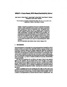


![[PDF]Read Foundations of Multithreaded, Parallel and ... - Google Sites](https://m.moam.info/img/260x300/pdfread-foundations-of-multithreaded-parallel-and-_6477ed2b097c474d228c956f.jpg)

![[PDF]Read Foundations of Multithreaded, Parallel, and ... - Google Sites](https://m.moam.info/img/260x300/pdfread-foundations-of-multithreaded-parallel-and-_6478a995097c474c228d61b4.jpg)

![[Read] Foundations of Multithreaded, Parallel, and ... - Google Sites](https://m.moam.info/img/260x300/read-foundations-of-multithreaded-parallel-and-goo_64785b53097c4796708cb848.jpg)
