Parallel Domain Decomposition Solver for

Parallel Domain Decomposition Solver for Adaptive hp Finite Element Methods J. T. Oden, Abani Patray, and Yusheng Fengy Texas Institute For Computational and Applied Mathematics University of Texas at Austin Austin,TX-78712 August, 1994 Abstract In this paper, the development and implementation of highly parallelizable domain decomposition solvers for adaptive hp nite element methods is discussed. Two level orthogonalization is used to obtain a reduced system which is preconditioned by a coarse grid operator. The condition number of the preconditioned system, for problems in two space dimensions, is proved to be bounded by Hp CH h (1 + logHp=h)(1 + logp) and C h (1 + logHp=h)(1 + logp), for different choices coarse grid operators, where H is the subdomain size, p is the maximum spectral order, h is the size of the smallest element in the subdomain, and C is a constant independent of the mesh parameters. The work here extends the work of Bramble et al. [4] on the h-version and Babuska et al. [3] on the p-version of the nite element method. A preliminary version of this solver was rst announced in [14]. Numerical experiments show fast convergence of the solver and good control of the condition number on a variety of discretizations. Director and Ernest and Virginia Cockrell Chair in Engineering y Graduate Research Assistant, TICAM

1

1 Introduction Adaptive hp nite elements, in which the spectral order and element size are independently varied over the whole domain, are capable of delivering solution accuracies far superior to classical h? or p?version nite element methods, for a given discretization size. Several researchers [2, 7, 18] have, in fact, shown that the reduction in discretization error with respect to number of unknowns can be exponential for general classes of elliptic boundary value problems, as opposed to the asymptotic algebraic rates observed for h or p-version nite element methods. Together with multiprocessor computing, these methods thus oer the possibility of orders of magnitude improvement in computing eciency over existing nite element models. A principal computational cost in any nite element solution is encountered in the solver. In a parallel computing environment, conventional direct solvers based on some variant of Gauss elimination are extremely inecient for the irregular sparse linear systems generated by adaptive hp discretizations. Further, as we discuss in the sequel, the linear systems are often very poorly conditioned, ruling out most standard iterative solvers. This feature also greatly degrades the solution obtained from direct solvers. Thus, ecient solvers meeting the twin criteria of being parallelizable and controlling the conditioning of the system, need to be developed. In recent years, very ecient parallel iterative solvers have been developed using the domain decomposition or substructuring ideas. These solvers are highly parallelizable and at the same time provide provably good control of the conditioning of the system. Bramble, Pasciak, and Schatz [4] developed the rst such solver for h?version nite element methods. They proved that the condition number of the linear system, generated by problems in two space dimensions, could be bounded by C (1 + log(H=h)2) where H is the subdomain size, h is the minimum element size within a subdomain and C is a constant independent of the mesh parameters. Dryja, Widlund and their coworkers obtained similar results using techniques based on the classical Schwartz alternating method [19, 8] and extended many of the results to three dimensions. Subsequently, Babuska, Craig, Mandel, and Pitkaranta [3] extended the method to p?version nite elements. Here again the condition number of the systems was proved to be bounded by C (1 + log2p). Bramble, Ewing and their coworkers [5] obtained sharper bounds for the hversion nite elements with local re nements in both two and three space dimensions. Mandel [10, 11] developed ecient preconditioners for p-version iterative solvers. Pavarino [17] obtained many theoretical results for the p?version with and without local re nements. More recently Ainsworth [1] 2

has extended the theoretical results of Bramble et al. to the hp-version on quasi-uniform meshes. Other than the preliminary announcement in [14], we know of no other parallel implementations of such solvers for hp-version nite element schemes. In this paper, we discuss a practical and ecient iterative solver for adaptive hp nite element discretizations. The solver is based on domain decomposition ideas and the preconditioned conjugate gradient method. We rst introduce a decomposition of the nite element space. Such decompositions may be automatically obtained by techniques discussed in Patra and Oden [16]. We then prove that, for problems in two space dimensions, the condition number of the preconditioned system can be bounded by C Hh (1 + logHp=h)(1 + logp) and C Hp h (1 + logHp=h)(1 + logp), for different choices of preconditioners, where H; p and h are the mesh parameters de ned before and C is independent of them. An implementation strategy and extensive numerical results complete the presentation.

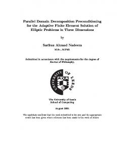
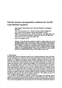
2 Condition Number Growth With h and p We begin our study of iterative solvers with a series of numerical experiments to demonstrate the growth of the condition number with the mesh parameters h and p for both uniform and non-uniform meshes. Using Poisson's equation on a rectangular domain as a test problem, we plot the growth in the condition number with changes in h and p. These calculations involve shape functions formed by standard tensor products of integrated Legendre polynomials. In Fig. 1, the growth with respect to uniform re nements and enrichments is plotted. In the next gure, Fig. 2, the growth of condition number over a sequence of adaptive hp meshes is plotted (see [15] for more examples and proofs on the condition number growth of several adaptive hp re nement patterns without domain decomposition treatment). In both cases the computed growth is seen to be very rapid.

3 Model Problem and Finite Element Spaces The solver will be discussed with respect to the model problem de ned below:

3

10000

uniform h uniform p

condition number

1000

100

10

1 0

200

400

600 degrees of freedom

800

1000

1200

Figure 1: Condition number growth for uniform h and p re nement for a model elliptic problem.

1

2

3

4

5

6

7

8

Spectral Order p

condition number

1E05 1E04 1E03 1E02 1E01 1 100

150 200 250 300 degrees of freedom

Figure 2: Typical computed results on condition number growth for a sequence of meshes produced by adaptive hp re nement. 4

Find u 2 V such that

B(u; v) = L(v) 8 v 2 V

(1)

where V = fv : v 2 H 1( ); v = 0 on @ g = (H01( )), and B(u; v) is the bilinear form on V characterizing a weak formulation of a two-dimensional second order elliptic PDE with Dirichlet conditions on the boundary @ and L is a continuous linear functional in V ; we require B(u; v) to be continuous on V , symmetric and coercive. Thus (1) is well posed and possesses a unique solution. In the theoretical developments given in Section 4, 5, 6, we focus on the Poisson problem for which

B(u; v) =

Z

ru rv dx

(2)

However, the general strategy has been successfully applied to more general boundary value problems. We consider a family G of partitions Ph of over which a sequence fV hpg of nite dimensional subspaces of V are constructed. For de niteness, but without loss of generality, we are concerned with approximation spaces based on the following structures: S1. is a connected domain ane equivalent, topologically, to a union of rectangles, and can be represented as the union of ND subdomains I such that

I \ J = ; I 6= J; and = [NI =1 I We denote HI = dia( I ); H = max HI I D

S2. The construction (in S1) de nes a family of coarse mesh partitions PH of which is assumed to be quasi-uniform. S3. Each subdomain is partitioned into a ner mesh of quadrilateral subdomains (the nite elements) !KI ; K = 1; 2; :::; NI ,

I = [NK=1!KI ; !KI \ !LI = ;; K 6= L and hIK = dia(!KI ) ; hI = min hI ; h = min h K K I I I

5

a

e 2

e2

(-1,-1) =

a

a 1 = (1,1)

1

a0

3

e3

e4

a

4

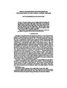
Figure 3: The master element The subpartitioning is quasi-uniform of size O(hI ) for each I. S4. Each quadrilateral element !KI is the ane image of a master element !b = [?1; 1]2. The master element has 9-nodal points: four vertices, ab1; ab2 ; ab3 ; ab4, four edge nodes eb1; eb2; eb3; eb4, and a centroid node, ab0 (see Fig. 3). Corresponding polynomial shape functions are constructed that fall into the following categories: Vertex Functions: These are the standard bilinear functions bi(; ) = 1 (1 )(1 ) i = 1; 2; 3; 4 (; ) 2 [?1; 1]2 4 ci(abj) = ij 1 i; j 4 Edge Functions: A polynomial function of degree pbs ; s = 1; 2; 3; 4, vanishing at the vertices, assigned to the edge nodes, e.g. bipb1 (; ) = ?21 (1 + )i() i = 2; :::; pb1 bipb2 (; ) = 21 (1 ? )i () i = 2; :::; pb2 bibp3 (; ) = ?21 (1 + )i() i = 2; :::; pb3 bipb4 (; ) = 1 (1 ? )i () i = 2; :::; pb4 2

6

Interior(Bubble) Functions: Corresponding to node ab 0, we introduce the functions

bbij (; ) = i()j () 2 i; j pb0

here

s

Z k () = 2k 2? 1 Pk?1 (s)ds ?1 with Pk?1 the Legendre polynomial of degree (k ? 1). We will denote the resulting space of functions spanned by the above shape functions by Qpb(!b ) where pb = max0i4 fpbig. Shape functions on each !KI will be polynomials of dierent degree at dierent nodes. We denote pIK = max. degree of the polynomial shape functions de ned on !KI and pI = max pI ; p = max p K K I I If FKI : !b ! !KI is an ane invertible map from !b to element !KI , then corresponding shape functions for !KI are of the form I c I ?1 Ki = i (FK ) ; I Ki = bipb (FKI )?1; etc. pj

j

and the restriction uIK of uhp 2 V hp to !KI is of the form, uIK = ubK (FKI )?1 S5. Interelement constraints are imposed so that, globally, V hp C 0( ); this can be accomplished using, for example, the schemes described in [7]. Throughout this investigation, we assume that conventions S1-S5 are in force, although the results are valid for much more general applications. The resulting structure admits the use of non-uniform mesh sizes and non-uniform distributions of spectral order p; thus, the methods under study here are true hp-version schemes. The particular mesh structure and p distribution is assumed to be given, and is generally determined by an adaptive strategy of the type given in [13, 18]. The situation of interest here, consistent with the conventions listed above, is illustrated in Fig 4. The domain is covered by a non-uniform hp 7

Ω2

Ω1

Ω4

Ω3 Ω

Ω

Ω

Figure 4: a) General hp mesh b) decomposition into 4 subdomains and c) a wire frame boundary of the subdomains. mesh, as indicated in Fig 4.a (dierent shadings suggesting dierent spectral orders p), supporting basis functions for the space V hp . This is partitioned into the the coarse mesh division PH consisting of of the ND subdomains

I , as shown in Fig 4.b. The inter-domain boundaries of the coarse mesh constitute a \wire frame" domain of functions spanned by vertex functions, as suggested in Fig 4.c. We distinguish between global basis functions corresponding to the vertices and edges of subdomain I and those interior to I : the vertices of I are hereafter called nodes; the edges and edge functions on @ I are called sides; vertices and edges interior to I on @!K n@ I retain the nomenclature, vertex and edge functions. Thus, there is a two-level hierarchy of functions de ning bases of the following spaces: Coarse Mesh: Nodal Functions: XIN = spanf(vertexfunctions)(aj ); aj 2 @ I g Side Functions

XIS = spanf(edgefunctions)(ej ); ej 2 @ I g 8

Interior Fine Mesh: Vertex Functions

XIV = spanf(vertexfunctions)(aj ); aj 2 I g Edge Functions

XIE = spanf(edgefunctions)(ej ); ej 2 I g Bubble functions

XIB = spanf(bubblefunctions)(a0j ); a0j 2 I g See Fig. 5. For each element !KI I , the element shape functions belong to the space 9 Qp (!KI ) = fu : u = u(x1; x2) : (x1; x2) 2 ! IK ; u = ub (FKI )?1; = ; (3) ub 2 Qpb(!b ); pb = pK = max0i4fpKi gg K

the resulting space of functions de ned on I by

9

> Fh;p( I ) = XIN + XIS + XIV + XIE + XIB > = hp p I = fv : v = v(x1; x2) = uj ; u 2 V ; vj! 2 Q (!K ); 1 I ND ; > (4) > ; 1 K NI ; h = (h1; h2; :::hN ); p = (p1; p2; :::pN )g K I

I

I

K

I

and, for a single element, we write

Fh;p(!KI ) = Qp (!KI ) K

(5)

It immediately follows that we may write (with obvious notations)

B(u; v) =

N X D

I =1

BI (u; v) =

N X N X D

I

I =1 K =1

9

BKI (u; v) 8 u; v 2 Fp;h( I )

(6)

V γ

iK

ωΚ

N S

Ω

i

E B

Figure 5: Decomposition of the nite element space; nodal (N) degrees of freedom are at nodes on subdomain I interfaces; side (S) are p-type degrees of freedom at sides between interface nodes; on the interior of the subdomains, vertices (V), edges (E) and bubbles (B) degrees of freedom are present.

4 Parallel Solver Algorithm

In terms of the decomposition of the nite element space introduced earlier, the bilinear form can be written as: N X B(uhp; uhp) = BI (uNhp + uShp + uVhp + uEhp + uBhp; uNhp + uShp + uVhp + uEhp + uBhp) D

I =1

where uhp is an arbitrary element of V hp. This results in a subdomain stiness matrix K I which contains submatrices associated with nodal (N), side (S) and internal (I) degrees of freedom. The internal degrees of freedom are further composed of vertex (V), edge (E) and bubble (B) degrees of freedom. Symbolically K I is of the form:

3 2 NN NS NI K I = 64 SN SS SI 75 IN IS II

3 2 VV VE VB II = 64 EV EE EB 75 BV BE BB

II represents the matrix corresponding to all internal degrees of freedom. 10

Level 1 Partial Orthogonalization Now if the local trial functions are chosen to satisfy the orthogonality condition

BKI ( j ; bk ) = 0 8 j 2 XiV + XiE + XiN + XiS ; bk 2 XiB (7) the element stiness matrix K elt and the submatrix corresponding to the

interior degrees of freedom reduce to

3 2 g g V V 0 elt V Eelt gelt EE gelt 0 75 K elt = 64 EV 0 0 BBelt

2 g VV 6 g II = 4 EV 0

3 VgE 0 7 g 0 5 EE 0 BB

g VgE represent modi ed blocks of the original matrix. We can where VgV ; EE; visualize this as a transformation of the bases of the spaces XIN ; XIS ; XIV ; XIE into spaces XfIN ; XfIS ; XfIV ; XfIE such that every element in the transformed space is orthogonal to every element in XiB in the inner product de ned by the bilinear form. This, in more conventional domain decomposition language, makes the spaces XfiN ; XfiS ; XfiV ; XfiE discrete harmonic to XiB . Level 2 Partial Orthogonalization If, in addition, the trial functions satisfy the orthogonality condition

BI;K (j ; 'k ) = 0 8j 2 XfIN + XfIS ; 'k 2 XfIV + XfIE + XIB

(8)

the resulting subdomain stiness matrices reduce to 3 2 g g 3 2 g g NN NS 0 V V V E 0 f = 64 EV g SS g 0 775 II g EE g 0 75 K I = 664 SN f 0 0 BB 0 0 II

g NS; g SN; g SS g are shared degrees of freedom among subdomains. where NN; Note that the rst orthogonality condition causes the orthogonalization of the bubbles with respect to the edges, vertices nodes, and sides while the second causes the orthogonalization of the interfaces with the interiors. The second orthogonalization makes the spaces XfIV + XfIE discrete harmonic with respect to XfIN + XfIS . The original nite element space is thus decomposed 11

into the sum,

Fh;p( I ) = (XfIN + XfIS ) (XfIV + XfIE ) XIB

(9)

and each u 2 Fh;p( I ) can be written as

u = (uN + uS ) (uV + uE ) uB

(10)

Remarks: 1. Implementation of the rst orthogonality condition can be done at the element level and is thus completely parallelizable. 2. Implementation of the second orthogonality condition involves modi g etc. which are of the form cation of NN etc. to NN N d I) g = X(NNI + NN NN D

I =1

d I is its where NNI is the NN -stiness matrix for domain I and NN modi cation produced by the partial-orthogonalization process. d I can be computed using only subdomain For each subdomain, NN data. Hence these computations are also parallelizable. 3. If an iterative solver (e.g. PCG) is used to solve the interface problem, these modi cations can then directly participate in the parallel matrixvector product that characterize these methods, and there is no need for assembly of these components. 4. The subdomain interior problems are now independent of the interface problem. The parallel domain decomposition algorithm is summarized as follows: Solution Algorithm 1. Partition the mesh into subdomains using any good decomposition algorithms(e.g. see Patra and Oden [16]).

12

2. Create subdomain approximations transforming the algebraic system at the element and subdomain levels to satisfy orthogonality conditions (7) and (8). This also creates independent subdomain problems and a global interface problem. 3. Solve the independent subdomain problems in parallel. 4. Solve the reduced preconditioned system by an iterative method (e.g. PCG) (using a preconditioner of the type described later by C in (18), (17) and (19). 5. Transform the solution of the reduced system to the original system for condition (8) at subdomain level and condition (7) at element level. 6. Solve the resulting system using parallel PCG iteration.

5 Condition Number Bounds For Problems in Two Dimensions With B(u; v) de ned by (2), we de ne norms and seminorms that we use in the sequel. The rst are the H 1 seminorms: juj21; = B(u; u) 8u 2 Fh;p( ) 9>> = juj21; = BI (u; u) 8u 2 Fh;p( I ) > (11) > juj21;! = BK (u; u) 8u 2 Fh;p(!KI ) ; I

I K

The weighted H 1( ) norm for domains of size H , i.e. dia( ) = H in two space dimensions, can be written as

jjujj21; = H12 jjujj2L2( ) + juj21;

(12)

The seminorms on the fractional spaces H 1=2(I ) = (H 0(I ); H 1(I ))1=2 and H01=2(I ) = (H 0(I ); H01(I ))1=2, respectively, where I = (a; b) RI , are given by

juj21=2;I

Z b Z b u(x) ? u(y) !2 dxdy = x?y a a 13

(13)

! ! u(x)2 dx + 2 Z b u(y)2 dy (14) x?a a b?y where \" means equivalent. These two norms are needed to characterize traces on element and subdomain boundaries. There are several technical results of independent interest on polynomial spaces that we shall use in our proof. For the sake of readability these are included in a separate section at the end of this article. For uhp 2 V hp , N N X X B(uhp; uhp) = BI (uhp; uhp) = uTI K I uI = uT Ku Z

b 2 2 0 jjujj1=2 juj1=2;I + 2 a

D

D

I =1

I =1

As demonstrated earlier, the matrices K I can be poorly conditioned. A matrix C is a preconditioner of K , and C I is a preconditioner of K I , if C is \spectrally close" to K (and C I to K I ), which means that

C ?1K I

(or C ?I 1 K I I I )

I (and I I ) being identity matrices. A bilinear form C on V hp V hp is a preconditioning form corresponding to B if constants m1 and m2 exist such that m1B(u; u) C (u; u) m2B(u; u)

u 2 V hp

(15)

and similar de nitions apply to BI . The justi cation of this nomenclature is due to the following properties: i.) Inequality (15) is equivalent to

m1uT Ku uT Cu m2uT Ku

8u 2 RI M ; M = dim(V hp)

ii.) If and are a generalized eigenfunction-eigenvalue pair de ned by

K = C with T C = 1 then is an eigenvalue of C ?1K and m1T K 1 m2T K 14

i.e.

m1min TminCmin m2max TmaxCmax

and

m1 max = (C ?1 K ) m2 min where (C ?1K ) is the condition number of C ?1K , which is hopefully close to unity. Thus, for any form C satisfying (15), the corresponding matrix C is a preconditioner of K , and the quality of the preconditioner is determined by the magnitude of the ratio of the constants (m1=m2) and its closeness to 1. Similar remarks apply to K I and C I . It is sucient to con ne our attention to preconditioners for the subdomain forms and matrices because of the following simple property: if u 2 V hp and if constants m1 and m2 exist such that

m1BI (u; u) CI (u; u) m2BI (u; u)

8I; I = 1; 2; ; ND

(16)

then

m1B(u; u) C (u; u) m2B(u; u) which follows by simply summing (16) over I . Thus, with N X C (u; u) = CI (u; u) D

I =1

we seek preconditioning forms C I with desirable properties for the hp-mesh constructions described earlier. Let XfIN ; XfIS ; XfIV ; XfIE and XIB denote the partially orthogonalized spaces introduced in Section 4 through matrix condensation (Schur complementation) steps described earlier. For Fh;p( I ) given by (9), denote dimXfIN = nN ; dimXfIS = nS ; dimXfIV = nV

dimXfIE = nE ; dimXIB = nB so that uhp can be represented in the form, n n n n n X X X X X uhpj = uN;j + uS;j + uV;j + uE;j + uB;j N

I

j =1

S

j =1

V

j =1

15

E

j =1

B

j =1

We also note that XfIS can be written as XfIS = [nk=1 XISk where nK is the number of edges on @ I and each XISk comprises of the orthogonalized side shape functions based on edge k. Clearly dimXISk pI ? 1. Then we de ne preconditioning forms on restrictions of functions in V hp to subdomain I by K

CI0(u; u)

9 > > = BI (uN;j ; uN;j ) + BI (uS;j ; uS;j ) = j =1 j =1 (17) n n n n n n X X X X X X > > +BI ( uV;j + uE;j + uB;j ; uV;j + uE;j + uB;j ) ; n X

n X

N

S

CI1(u; u)

j =1

j =1

i=j

j =1

j =1

B

E

V

B

E

V

j =1

9 > > = BI ( uN;j ; uN;j ) + BI (uS;j ; uS;j ) = j =1 j =1 j =1 (18) n n n n n n X X X X X X > > +BI ( uV;j + uE;j + uB;j ; uV;j + uE;j + uB;j ) ; n X

n X

n X

S

N

N

V

E

j =1

B

j =1

V

i=j

E

j =1

j =1

B

j =1

9 > > CI2(u; u) = BI ( uN;j ; uN;j ) + BI ( uS;jk ; uS;jk ) > = j =1 j =1 j =1 j =1 k=1 (19) n n n n n n X X X X X X > > +BI ( uV;j + uE;j + uB;j ; uV;j + uE;j + uB;j ) > ; j =1 j =1 i=j j =1 j =1 j =1 n X

n X

n X

V

pX ?1

K

N

N

E

pX ?1

k

B

k

V

E

B

C 0I is computationally much simpler to implement than C 1I and C 2I . However unlike C 1I it is dicult to establish reasonable bounds on the performance of C 0I . Another choice of preconditioner for hp nite elements can

be found in Ainsworth [1]. To establish properties of C 1I and C 2I we rst lay down several basic lemmas. Hereafter, we denote HI ; hI , and pI by simply H; h, and p. Note that in actual implementation only the rst two terms are used on the reduced system as a preconditioner.

Lemma 1 Let conventions S1-S5 hold and let Fh;p( I ) be the nite element space de ned in (4). If

i) BI (u; v) = 0 ii) BI (u; v) = 0

8u 2 XfN + XfS ; v 2 XfV + XfE + X B 8u 2 X B ; v 2 XfN + XfS ; v 2 XfV + XfE ; 16

then for any u 2 Fh;p( I ), BI (u; u) k CIk (u; u) k = 1; 2 where C kI is de ned in (18) and (19) 8 Hp < c for k = 1 k = : Hh c h for k = 2

Proof: Since n n n n n X X X X X BI (u; u) = BI ( uN;j + uS;j + uV;j + uE;j + uB;j ; N

n X

S

j =1

n X

V

j =1

n X

E

j =1

n X

B

j =1

n X

j =1

uS;j + uV;j + uE;j + uB;j ) j =1 j =1 j =1 j =1 n n n n X X X X BI ( uN;j ; uN;j ) + BI ( uS;j ; uS;j ) j =1 j =1 j =1 j =1 n n n n n n X X X X X X + BI ( uV;j + uE;j + uB;j ; uV;j + uE;j + uB;j ) j =1 j =1 j =1 j =1 j =1 j =1 n n X X +2BI ( uN;j ; uS;j ) j =1 j =1 N

j =1

=

uN;j +

V

S

S

N

N

B

E

V

S

E

B

V

E

B

S

N

Now, applying the Cauchy-Schwartz inequality and the arithmetic geometric n n X X mean inequality on the term 2BI ( uN;j ; uS;j ), we have N

S

j =1

n X

2BI ( uN;j ; N

j =1

j =1

n X

n X

n X

X

nS 1 2 N;j )) ( I (

n X

uS;j ) 2(BI ( uN;i; u B uS;j ; uS;j )) 12 j =1 j =1 j =1 j =1 j =1 n n n n X X X X BI ( uN;j ; uN;j ) + BI ( uS;j ; uS;j ) N

N

S

N

N

j =1

S

j =1

S

S

j =1

j =1

n n X X Aplying the same strategy on BI ( uS;j ; uS;j ), we have j =1 j =1 0 1 n n X n n n X X X X BI (uS;j ; uS;k )A BI ( uS;j ; uS;j ) = BI (uS;j ; uS;j ) + @ S

S

j =1

S

j =1

S

S

S

S

j =1 k=1

j =1

0n n 1 X X Let us examine at the term @ BI (uS;j ; uS;k )A . S

S

j =1 k=1

17

j 6=k

j 6=k

For each non-zero BI (uS;i; uS;j ), this leads to

BI (uS;i; uS;j )i6=j BI (uS;i; uS;i) 21 BI (uS;j ; uS;j ) 12 21 (BI (uS;i; uS;i) + BI (uS;i; uS;i)) Hence ( Thus,

n X n X S

S

j =1 k=1

BI (uS;j ; uS;k ))j6=k (nS ? 1)

n X S

k=1

BI (uS;k ; uS;k )

(20)

n X

n X

n X

n X

j =1

j =1 n X

j =1

j =1

BI (u; u) 2(BI ( uN;j ; uN;j ) + 2( BI (uS;j ; uS;j ) + (nS ? 1) N

N

S

S

BI (uS;j ; uS;j ))

n n n n n X X X X X +BI ( uV;j + uE;j + uB;j ; uV;j + uE;j + uB;j ) j =1 j =1 j =1 j =1 j =1 j =1 1 2nS CI (u; u) V

E

B

V

B

E

Note that

nS nK (pI ? 1) For problems in two dimensions, under assumptions S1-S5 on the mesh, nK can be bounded above by

q nK cpnelt = c H 2=h2 = c Hh

where nelt is the number of elements in the subdomain and c is a small constant independent of H and h. This leads to 1(u; u) BI (u; u) c Hp C I h n n X X To develop the bound on C 2I we rewrite BI ( uS;j ; uS;j ) j =1 j =1 p ? 1 p ? 1 n n XX XX uS;jk ). Applying the Cauchy-Schwartz and uS;jk ; as BI ( S

K

k

k=1 j =1

K

k

k=1 j =1

18

S

arithmetic-geometric mean inequalities as before leads to ?1 pX ?1 ?1 pX ?1 n pX n pX n X X X BI ( uS;jk ; uS;jk ) = BI ( uS;jk ; uS;jk ) j =1 j =1 k=1 j =1 k=1 j =1 k=1 pX ?1 pX ?1 n X n X + (BI ( uS;jk ; uS;jl)k6=l j =1 j =1 k=1 l=1 pX ?1 pX ?1 n X BI ( uS;jk ; uS;jk ) j =1 j =1 k=1 pX ?1 pX ?1 nX +(nK ? 1) BI ( uS;jk ; uS;jk ) K

k

K

k

k

k

K

K

k

k

K

k

k

K

k

k

K

j =1

j =1

k=1

Thus, n X

n X

n X

j =1

j =1

k=1

BI ( uS;j ; uS;j ) nK S

S

and

Lemma 2 De ne

K

BI (

pX ?1 k

j =1

uS;jk ;

pX ?1 k

j =1

uS;jk )

BI (u; u) c Hh CI2(u; u)

n 2 X 1 juj21;

uN;j j =1 1;

n X juS;j j21; 2 juj21;

N

I

I

S

j =1

I

I

Then under the assumptions of Lemma 1 and

1 C (1 + log Hp h) 2 C (1 + log Hp h )(1 + logp)

where C is independent of H,h and p.

Proof: The proof essentially comprises of computing bounds on the energy ratios of the components of the preconditioner and u 2 Fh;p( I ). The proof 19

is largely inspired by similar results for the p version in Babuska et al.[3] and the h version in Bramble et al.[4]. Let xj denote the coordinates of a node on the interface and let j denote the rst order Lagrange shape function associated with xj . Clearly j 2 Fh;p( I ). Hence j can be decomposed as

j =

n X N

jk=1

jk uN;jk

n X V

jk=1

( jk uV;jk +

n X E

jl=1

jl uE;jl)

n X B

jm=1

jmuB;jm

(21)

because of the discrete harmonic nature of uN;j . Thus, n n n n X X X X BI ( uN;j ; uN;j ) BI ( uN;j (xj )j ; uN;j (xj )j ) j =1 j =1 j =1 j =1 n X C jj uN;j jj2L1 ( ) j =1 C jjujj2L1( ) C (1 + log Hph )jjujj21;

where we have applied Theorem 2 (see Section 7) to the second term. Let u be an average value for u. From the previous inequality and Poincare's inequality, 9 n n X X > Hp 2 > BI ( uN;j ? u; uN;j ? u) C (1 + log h )jju ? ujj1;

> > j =1 j =1 C (1 + log Hph )(juj21; + H12 jju ? ujj2L2( )) >= (22) > 2 2 C (1 + log Hph )(juj21; + C1 H juH?u2 j1 ) >>> ; C (1 + log Hph )juj21;

N

N

N

N

N

I

I

I

N

N

I

I

I

;

I

I

I

Hence

1 C (1 + log Hp h)

Now de ne

n X u1 = u ? uN;i i=1 The function u1 is zero at all the vertices xi on @ I . By the triangle inequality, 2 ju1j21; C (1 + log Hp h )juj1;

N

I

I

20

In Fh;p( I ),

1 2 ku1 k1;

) ku1kL1 (@ ) C ku1kL1 ( ) C (1 + log Hp h I

I

I

using Theorem 2. Let iK = @ I \ !KI such that I = [NK=1 !IK . By Lemma 7 and the trace theorem, X 2 ju1j221 ;@ + C (1 + log p) ku1k2L1(@ ) 0 ku1k 21 ; I

K

iK

I

I

C1 ku1k21; + C (1 + log p) ku1k2L1(@ ) I

I

C1 ku1k21; + C (1 + log p) kuk2L1 (@ ) I

I

2 C1 ku1k21; + C2(1 + log p)(1 + log Hp h ) kuk1;

I

I

2 C (1 + log p)(1 + log Hp h ) kuk1;

I

By Lemma 9, 9 u~S;j 2 XfS (XfV + XfE + XB ) such that u~s = u1 on @ I and X ku~S;j k21; C 0 ku1k221 ; K

I

iK

2 C (1 + log p)(1 + log Hp h ) kuk1;

I

Let uS;j 2 XfS , then uS;j = u~S on @ I , and (uS;j ? u~S;j ) 2 XfV + XfE + XB From assumption (i) and (ii) of Lemma 1, we have Hence,

BI (uS;j ; uS;j ) BI (~uS;j ; u~S;j ) juS;j j21; C ju~S;j j21;

C ku~S;j k21;

C (1 + log p)(1 + log Hph ) juj21;

I

I

I

I

Applying a procedure similar to (22), we nd that

2 ) j u j juS;j j21; C (1 + log p)(1 + log Hp 1;

h I

21

I

(23)

Thus,

2 C (1 + log p)(1 + log Hp h)

Combining the result in Lemmas 1 and 2 gives the nal major result:

Theorem 1 If the conditions in Lemmas 1 and 2 hold, then the condition number of the system ( = (C ?1 B )) satis es 8 N > X Hp Hp 1 > > < C h (1 + log p)(1 + log h ) for C = I =1 C I > N H (1 + log p)(1 + log Hp ) for C = X > C C 2I > : h h I =1 D

D

where C is independent of H,h and p.

Remarks: As we shall see in the next section on numerical experiments this

bound is quite pessimistic, and rarely seen in practice. The linear growth in condition number with Hp h as the above bounds seem to suggest is also not seen. We note here that Ainsworth's preconditioner has a sharper bound on 2 the condition number(O(1 + log Hp h ) ). However the extremely complicated nature of the sequence of inner products used to de ne the preconditioner, make it more expensive to implement.

6 Numerical Results The numerical results presented in this section are obtained by applying the strategies described in Section 4 to the Poisson's problem (?u = f ), in two dimensions with a unit square. Condition number estimates of the reduced system, iteration counts of the iteration scheme, and parallel eciency of the domain decomposition algorithm are presented. The results show that the conditioning of the reduced system is dramatically improved, fast convergence is achieved in terms of low iteration counts for the iteration scheme, and reasonably good parallel eciencies are obtained for highly nonuniform adaptive hp meshes. We compare the performance of the preconditioners introduced in the previous sections (17), (18), and (19), which we shall denote as HPP0, HPP1, 22

100000 HPP0 HPP1 HPP2 original system

condition number

10000

1000

100

10

1 1

2

3

4 spectral order p

5

6

7

Figure 6: Control of condition number with increase in p.Problem was decomposed into 4 subdomains with H=h = 2. and HPP2 respectively, with the original system without any preconditioning. The condition number estimates are calculated using an extended version of Lanczos' connection, which is derived in [15], to Preconditioned Conjugate Gradient (PCG) methods. In Fig. 6 the control of conditioning by the dierent preconditioning strategies for increasing spectral order is shown. All the preconditioners appear to control the conditioning quite well. In Fig. 7, the condition number is plotted against spectral order p, for the case of 8-subdomains with H=h = 4. It is evident that the condition number the reduced system is less than the estimate from Theorem 1. In Figure 8, the condition number vs. ratio H=h is plotted for the case of 4subdomains with p = 2. Notice that the condition number of the reduced system, after applying HPP1 preconditioner, is well within the the theoretical bounds; while the condition number of the reduced system, after applying HPP0 preconditioner, seems to have a larger growth rate. The expected linear growth with H=h is not seen in practice at least for H=h 8. In Table 1, the condition number estimates and iteration counts of a 4subdomain system with HPP0 preconditioner for various spectral order p and ratios of subdomain size over mesh size H=h are listed. The condition number estimates for the same system but with HPP1 and HPP2 preconditioning are shown in Tables 3 and 4. For large p (p 4) HPP2 appears to improve the 23

10000 C*p(1+log p)(1+log 4p) HPP0 precond. HPP1 precond.

condtion no.

1000

100

10

1 1

2

3

4

5

6

spectral order p

Figure 7: Plot of condition number: 8 subdomains with H=h = 4.

1000 C*(H/h)*(1+log H/h) HPP0 HPP1

condition no.

100

10

1 1

2

3

4

5

6

7

8

H/h

Figure 8: Plot of condition number: 4 subdomains with p = 2. 24

Spectral Order p 1 2 3 4 5 6 7 8

Figure 9: hp Adaptive Mesh (dof=660). conditioning. For the system resulting from a 4-subdomain decomposition, the HPP0 preconditioner appears to works as well as the HPP1 preconditioner for a constant ratio of H=h. However, the HPP0 preconditioner cannot control the conditioning of the system as the ratio H=h increases. The HPP1 preconditioner, on the other hand, improved the conditioning of the reduced system as predicted in the theory. For the reduced system resulting from a 8-subdomain decomposition, there is a large dierence in condition number between using HPP0 and HPP1 preconditioners. The results in Tables 2 and 5 show that the condition number of the reduced system, after applying the HPP1 preconditioner, is much smaller than that after applying the HPP0 preconditioner. Table 6 displays the eectiveness of the HPP1 preconditioner for an hp adaptive mesh.The mesh used in this calculation is shown in Figure 9. This mesh is obtained using an hp adaptive strategy described in [13] and corresponds to a non-homogeneous Poisson problem with exact solution u = tan?1(x + y ? x0)x(1 ? x)y(1 ? y) for = 50. The condition number and iteration counts of the reduced system, after applying the HPP1 preconditioner are compared with that those applying HPP0 preconditioner. 25

p 1 2 3 4 5 6 7 8

H/h=1 Cond# Itr# 1.00 1 (5.07) 3.45 3 (.235E2) 5.19 4 (.187E3) 7.29 7 (.762E3) 9.13 9 (.227E4) 11.14 11 (.560E4) 12.96 13 (.127E5) 15.07 15 (.242E5)

H/h=2 Cond# Itr# 2.45 3 (11.98) 4.65 7 (.594E2) 5.93 11 (.326E3) 8.63 15 (.130E4) 10.09 19 (.341E4) 12.63 22 (.862E4) 17.52 23 (.170E5) 21.30 25

H/h=4 H/h=8 Cond# Itr# Cond# Itr# 5.50 7 12.28 15 (.362E2) (.123E3) 6.83 15 12.53 28 (.838E2) 7.55 21 (.399E3) 9.91 26

Table 1: Condition number estimates and iteration counts for system decomposed into 4 subdomains and preconditioned with an HPP0 type preconditioner. Condition numbers for the original system with no preconditioning are listed in parentheses. Two types of decompositions are attempted, a strip type decomposition in which the domain is decomposed into strips(called a \horizontal decomposition" in the table), and a second one in which the subdomains are more compact(called a \cross decomposition" in the table). H=h for the \cross decomposition" is about half that of the \horizontal decomposition". The performance of HPP1 preconditioner is quite dramatic. The number of iterations is 5 for HPP1 as opposed to 26 for the HPP0. Further, use of a HPP0 preconditioner on the unreduced problem did not converge and the condition number was estimated to be O(104). Comparing the two decompositions, it is also apparent that the smaller the ratio H=h, the better the conditioning of the reduced system. We now try dierent spectral orders p, on an uniform grid of 64 elements. In Fig. 10, both iteration counts and condition number estimates are plotted against p (ranging from 2 to 8). The condition number is controlled to remain under 16. Figure 11 shows the residual and condition number estimation 26

p 1 2 3 4 5 6

HPP0 HPP1 HPP2 dof Cond # Itr # Cond # Itr # Cond # Itr # 81 7.90 21 1.00 1 1.00 1 289 11.44 23 5.00 28 5.00 28 625 12.16 36 7.02 30 7.15 31 1089 14.69 43 10.08 37 9.77 35 1681 15.63 43 12.20 38 11.6 36 2041 18.85 48 15.00 44 13.65 39

Table 2: Condition number estimates and iteration counts for the 8subdomain system (H=h = 4).

H/h=1 p Cond# Itr# 1 1.00 1 (5.07) 2 3.45 3 (.235E2) 3 5.19 4 (.187E3) 4 7.29 7 (.762E3) 5 9.13 9 (.227E4) 6 11.14 11 (.127E5) 7 12.96 13 (.127E5) 8 15.07 15 (.242E5)



Table 3: Condition number estimates and iteration counts for system decomposed into 4 subdomains and preconditioned with an HPP1 type preconditioner. Condition numbers for the original system with no preconditioning are listed in parentheses. 27

p 1 2 3 4 5 6 7 8

H/h=1 Cond# Itr# 1.00 1 (5.07) 3.45 3 (.235E2) 5.19 4 (.187E3) 6.72 5 (.762E3) 8.07 6 (.227E4) 9.29 7 (.127E5) 10.4 8 (.127E5) 11.44 8 (.242E5)



Table 4: Condition number estimates and iteration counts for system decomposed into 4 subdomains and preconditioned with an HPP2 type preconditioner. Condition numbers for the original system with no preconditioning are listed in parentheses.

p 1 2 3

dof 289 1089 2401

HPP0 HPP1 Cond # Itr # Cond # Itr # 16.77 32 1.00 1 20.74 41 4.81 28 21.37 44 6.72 30

Table 5: Condition number estimates and iteration counts for the 8subdomain system (H=h = 8). 28

Cross Decomposition HPP0 HPP1 H/h Cond # Itr # Cond # Itr # 8 8.25 25 5.05 21 Horizontal Decomposition HPP0 HPP1 H/h Cond # Itr # Cond # Itr # 32 9.50 30 5.20 21 Table 6: Condition number estimates and iteration counts for an adaptive hp mesh(dof=660, p=6).

20 iteration count cond. no. estimate 18

iteration count/condition no.

16

14

12

10

8

6

4

dof=81(17)

2 2

dof=1089(65) 3

4

5 spectral order p

6

7

8

Figure 10: Iteration counts and condition numbers for HPP1 preconditioner for dierent spectral orders (4 sub-domain).

29

1e+10 ’p8.dat’ ’p8.dat’ ’p8b1.dat’ ’p8b1.dat’

condition no./residual

1

1e-10

1e-20 0

50

100

150 no. of iteration

200

250

300

Figure 11: Comparison of HPP1 solver with conventional Jacobi iterative solver.

cpu time in seconds/processor

100

(325)

10

(169)

(91)

1 2

3

4

5 no. of proc

6

7

Figure 12: Parallel eciency on Intel iPSC/860. 30

8

against iteration count for HPP1 and HPP0. Figure 12 demonstrates the parallel eciency of the solver on an Intel iPSC/860 for 2,4 and 8 processors. We observe that the speedup is almost 5 from 2 to 4 processors, and 2.5 from 4 to 8 processors. This is because of the reduction in block size . The computational eort in \partial orthogonalization", ensuring that conditions (i) and (ii) in Lemma 1 are satis ed, reduces steeply with block size leading to the very high speedup. However reducing the block size also increases the size of the reduced system and communication overheads in a parallel environment. This raises the intriguing possibility of nding an optimal block size for such problems.

7 Auxiliary Results In this section we list some technical results which are used in the proofs in Section 5. Most of these are extensions of standard results available in the literature for the h or p version nite element method. Alternate proofs of some of these results may be found in [1].

Lemma 3 (Bramble and Xu [6]) If is a bounded domain in RI 2 and @

is Lipschitz continuous, then for any 2 (0; 1), and any w 2 W 1;1 ( ), jjwjjL1( ) C (jlogj 12 ( H12 jjwjjL2( ) + jwj1; ) 12 + (jjwjjL1( ) + H jjrwjjL1( ))) where H = dia( ), and C is a constant independent of H .

(24)

Proof: This result follows immediately from a result of Bramble and Xu [6]

and Xu[20] after a straightforward scaling with respect to H . The next result is the classical Markov's inequality for polynomials.

Lemma 4 (Markov) If v is polynomial of degree p on I = [-h,h], then 0(x)j p max jv (x)j max j v I h I 2

Proof: See page 40 of Lorentz [9]. 31

(25)

Lemmas 3 and 4 lead to a very useful bound on the maximum value of the function in terms of the H 1( ) norm.

Theorem 2 Let u 2 Fh;p( I ), then jjujj2L1( ) I

Hp C 1 + log h jjujj21;

I

(26)

where H = dia( I ); h = minK dia(!K ), p is the maximum order of polynomial in !K and C is independent of H, p and h.

Proof:

v !2 !2 u u t @u + @u jjrujjL1( ) = max x @x1 @x2 ! @u + @u max x @x1 @x2 I

Applying Markov's inequality to

@u @u @x1 ; @x2 , we

obtain

@u p2 max ju(x ; x )j max 1 2 x1 @x1 h x1 @u p2 max ju(x ; x )j max 1 2 x2 @x2 h x2 Hence i.e.

jjrujjL1 2 ph max x ju(x1; x2)j 2

jjrujjL1( ) 2 ph jjujjL1( ) 2

I

I

Lemma 3 holds 8 2 (0; 1). Choosing as = 4Cph2H 32

Since p 1 and H h, it follows that 2 (0; 1) for all C = C0 1=4. Then jlogj1=2 = j4logC + 2log hp + logH j1=2 Lemma 3 thus leads to

1=2jjujj 1 + h (1+ 2Hp )jjujj 1 ) jjujjL1( ) C (j4logC0+2log pH j L ( ) H ( ) h 4C p2H h 2

I

0

I

or

I

1 + 2 jjujj 1 ) 1=2jjujj j jjujjL1( ) C (j4logC + 2log pH 1; + L ( ) h 4 where = Hp2 =h. Now > 1 since H=h 1 and p 1. Thus I

I

and

1 + 2 3 4 4

1=2 jjujjL1( ) C1(j4logC0 + 2log pH h j jjujjH 1( )) I

where

I

I

C1 =

The result follows.

C

1 ? 1+2 4

4C

Lemma 5 Let f be a continuous function on I = (a,b), let I be partitioned into n subintervals Ik : I = \nk=1 Ik . Then n X k=1

jfk j21=2;I jf j21=2;I k

(27)

where fk = f jI

k

Proof: By de nition,

Z Z f (x) ? f (y) !2 = I I dxdy x?y Breaking up the integrals using I = [k Ik and noting that the integrands are positive, we have Z Z f (x) ? f (y) !2 Z Z f (x) ? f (y) !2 2 dxdy + dxdy + ::: jf j1=2;I = I I x?y x?y I1 I2 1 1

jf j21=2;I

33

+

! n f (x) ? f (y) 2 dxdy X jfk j21=2;I x?y k=1

Z Z I

I

n

k

n

Lemma 6 Let Zp = fu 2 Pp(Ik ); Ik = [?h; h]ju(?h) = u(h) = 0; 8p > 0g. Then

2 0 jjujj1=2;I

k

juj21=2;I + C (1 + logp)jjujj2L1(I ) k

k

(28)

Proof: By de nition,

Z h u(x)2 Zh 2 ( x + h )dx + 2 ( hu(?y)y )dy ?h ?h We need to bound the last two integrals. Breaking up the second integral into two parts Z h u(x)2 Z h u(x)2 Z h? 2 u(x)2 ( ( ) dx = ) dx + ( h ? x )dx ?h ?h h ? x h? 2 h ? x 2 0 jjujj1=2;I

k

= juj21=2;I + 2

h

p

h

p

Since u 2 Zp(Ik ) we have for any x 2 Ik ,

u = (h ? x)v where v 2 Pp?1(Ik ). Further u0 2 Pp?1(Ik ). Hence we have from Markov's inequality ju(x)j (h ? x) max x jv (x)j 0 C (h ? x) max x ju (x)j 2 C (h ? x) ph jjujjL1(I ) Applying this to the rst part gives 0Z 1 Z h u(x)2 Z h? 2 1 4 h p (h ? x) h2 dx + ( )dx C jjujj2L1(I ) @ ( h ? x )dxA ?h h ? x ?h h? 2 k

h

p

k

h

p

Computing the integrals Z h u(x)2 ( h ? x )dx C jjujj2L1(I )f 21 + 2logp + log2g ?h C (1 + logp)jjujj2L1 (I ) k

k

The rst integral can be bounded similarly. 34

Lemma 7 Let Fh1;p(I ) = [k Zp ; I = (?H; H ); I = [k Ik . If u 2 Fh1;p(I ) such that uk = ujI then k

k

X k

2 0 jjuk jj1=2;I

k

juj21=2;I + C (1 + logp)jjujj2L1(I )

(29)

Proof: Combining the previous two lemmas, we have X X 2 2 2 0 jjuk jj1=2;I = (juj1=2;I + C (1 + logp)jjujjL1 (I )) k k juj21=2;I + C (1 + logp)jjujj2L1(I ) k

k

k

That completes the proof. We now present two simple lemmas on extensions of functions de ned on the boundaries of subdomains into their interior. These will allow us to bound energies of such extensions in terms of the values of these functions on the subdomain interfaces. The rst is a result introduced by Babuska and Suri [2] on a single master element. The second is an extension of this to the hp nite element spaces de ned on subdomains.

Lemma 8 (Babuska and Suri [2]) Let the square S = f(x; y) : jxj 1 and jyj 1g and f such that f (A) = f (B ) = f (C ) = f (D) = 0 where A; B; C; D are the vertices of the square. Further, let fi = f j ; i = 1; 2; 3; 4 where i denote the sides of the square. Now let f1 2 Pp( 1) and f2 = f3 = f4 = 0 Then there exists U 2 Pp(S ) such that U = f on @S and jjU jj21;S C 0jjf1jj212 ; 1 i

where C is independent of p and f .

Proof: This is a special case of the more general result in Babuska and Suri [2] where fi = 6 0; i = 2; 3; 4. Lemma 9 (Extension Theorem) Let SIK 2 Pp ( IK ), where IK = @ I \

@!K , and let the side shape functions on @ i vanish at all nodal points N = A; B; ; 2 @ I : SIK (A) = SIK (B ) = = 0. Then there exists a U 2 Fh;p( I ) where U j = SIK such that X (30) jjU j j21; C kSI k221 ; K

IK

I

C

35

K 2 0 kS k 21 ;@

IK

I

(31)

C

D

B

γ

A ω

iK

K

Figure 13: Illustration of the Extension Function (See Fig. 13 for an illustration).

Proof: Consider an extension uK 2 Qp (!KI ) such that k

uK j = SIK

on IK

IK

By Lemma 8,

kuK k1;! C 0 kS k 21 ;

IK

K

Now construct U on I by de ning

8 < uK (x; y) 2 ! K U =: 0 (x; y) 2 i n 2 ! K where !K are elements such that @!K T @ I 6= ;. Then

kU k21; = I

X K

Then 36

kuK k21;!

K

kU k21; C PK 0 kSik221 ; C PK 0jjSijj221 ;@

i

iK

I

8 Conclusions In this paper, a parallel domain decomposition solver for adaptive hp nite element methods for two dimensional elliptic problems is developed and analyzed. The condition number for the solver is proved to be bounded by C Hph (1+log p)(1+ log Hph ) and C Hph (1+log p)(1+log Hh ) for dierent choices of preconditioners. The factor Hh and Hp h in these estimates render them sub-optimal. In practical calculations, we generally take p 9 and H=h 4. For our approach results of estimated condition number and iteration counts show that the conditioning of the reduced system is controlled, and fast convergence is achieved as predicted in the theoretical analysis. Parallel results are obtained on an Intel iPSC/860. Good parallel eciencies are demonstrated.

Acknowledgments The support of this work by ARPA under contract no. DABT63-92-C0042 is gratefully acknowledged. We also wish to acknowledge Dr. Mark Ainsworth's suggestions for improving earlier drafts of this work.

References [1] M. Ainsworth, \A Preconditioner Based on Domain Decomposition of hp Finite Element Approximation on Quasi-Uniform Meshes," Mathematical and Computer Science Technical Reports, University of Leicester, no. 16, 1993. [2] I. Babuska and M. Suri, \The h-p version of the Finite Element Method With Quasiuniform Meshes" Mathematical Modelling and Numerical Analysis, Vol. 21, no. 2,1987, pp. 199-238. [3] I. Babuska, A. Craig, J. Mandel, and J. Pitkaranta, \Ecient Preconditioning for the p Version Finite Element Method in Two Dimensions," SIAM J. Numer. Anal, Vol 28, No. 3, pp. 624-661, June 1991. 37

[4] J. Bramble, J. Pasciak, and A. Schatz, \The Construction of Preconditioners for Elliptic Problems by Substructuring I," Math. Comp. 47, no. 175 (1986), pp. 103-134 [5] J. H.Bramble, R. H. Ewing, R. H. Parashkevov, and J. Pasciak, \Domain Decomposition For problems with Partial Re nement," SIAM J. Sci. Sta. Comp., Vol. 13, No. 1., 1992, pp. 397-410. [6] J. H. Bramble and J. Xu, \Some Estimates for a Weighted L2 Projection," Math. Comp., 56(1991), pp.463-476. [7] L. Demkowicz, J. T. Oden, W. Rachowicz and O. Hardy, \Toward A Universal hp Adaptive Finite Element Strategy, Part 1. Constrained Approximation and Data Structure," Comput. Methods. Appl. Mech. and Engg., 77(1989), pp.79-112. [8] M. Dryja, \An Additive Schwarz Algorithm for Two- and Three Dimensional Finite Element Elliptic Problem," In T. Chan, R. Glowinski, J. Periaux, and O. Widlund, editors, Domain Decomposition Methods, SIAM, Philadelphia, 1989. [9] G.G. Lorentz, \Approximation of Functions," Chelsea Publishing Co. New York, N.Y.,1966 [10] J. Mandel, \Ecient domain decomposition preconditioning for the pversion nite element method in three dimensions," Technical report, University of Colorado at Denver, 1989. [11] J. Mandel, \Iterative solvers by substructuring for the p-version nite method," Comput. Meth. Appl. Mech. Engg, 80(1990), pp117-128. [12] J. Mandel, \Two level Domain decomposition preconditioning for the p-version nite element method in three dimensions," Int. J. Numer. Meth. in Engg.,29(1990),pp.1095-1108. [13] J. T. Oden, Abani Patra, and Y. S. Feng, \ An hp Adaptive Strategy," Adaptive, Multilevel, and Hierarchical Computational Strategies, A. K. Noor(ed).AMD-Vol. 157, 1992, pp. 23-46. [14] J. T. Oden, Abani Patra, and Y. S. Feng, \Domain Decomposition Solver For Adaptive hp Finite Elements" VIIth International Conference on Domain Decomposition, State College, Pennsylvania, October, 1993. [15] J. T. Oden and Y. S. Feng, \Optimal hp Finite Element Methods; Part 1: Conditioning Analysis, Preconditioning Strategies, and Construction of Optimal Trial Spaces" (In preparation) 38

[16] A. Patra and J. T. Oden, \Problem Decomposition for Adaptive hp Finite Element Methods," (submitted). [17] L. Pavarino, \Domain Decomposition For p version Finite Element Methods," Ph. D. Dissertation, Courant Institute, New York University, 1993. [18] W. Rachowicz, J.T. Oden and L. Demkowicz, "Toward A Universal hp Adaptive Finite Element Strategy; Part 3: Design of hp Meshes," Comput. Meth. Appl. Mech. and Engg., 77(1989), pp.181-212 [19] O.B. Widlund, \Iterative Substructuring Methods: Algorithms and Theory for Elliptic Problems in the Plane," In R. Glowinski, G.H. Golub, G.A. Meurant, and J. Periaux, editors, First International Symposium on Domain Decomposition Methods for Partial Dierential Equations, SIAM, Pheladelphia, PA, 1988. [20] J. Xu, \Theory of Multilevel Methods," Pennsylvania State University, Dept. of Mathematics, Report NO. AM 48, 1989.

39