Parallel Sn Sweeps on Unstructured Grids

NUCLEAR SCIENCE AND ENGINEERING: 150, 267–283 ~2005!

Parallel Sn Sweeps on Unstructured Grids: Algorithms for Prioritization, Grid Partitioning, and Cycle Detection Steven J. Plimpton,* Bruce Hendrickson, and Shawn P. Burns Sandia National Laboratories, Albuquerque, New Mexico 87185

William McLendon III Sandia National Laboratories, Albuquerque, New Mexico 87185 and Texas A&M University, Department of Computer Science, College Station, Texas 77843-3112

and Lawrence Rauchwerger Texas A&M University, Department of Computer Science, College Station, Texas 77843-3112 Received September 6, 2002 Accepted September 14, 2004 Abstract – The method of discrete ordinates is commonly used to solve the Boltzmann transport equation. The solution in each ordinate direction is most efficiently computed by sweeping the radiation flux across the computational grid. For unstructured grids this poses many challenges, particularly when implemented on distributed-memory parallel machines where the grid geometry is spread across processors. We present several algorithms relevant to this approach: (a) an asynchronous message-passing algorithm that performs sweeps simultaneously in multiple ordinate directions, (b) a simple geometric heuristic to prioritize the computational tasks that a processor works on, (c) a partitioning algorithm that creates columnarstyle decompositions for unstructured grids, and (d) an algorithm for detecting and eliminating cycles that sometimes exist in unstructured grids and can prevent sweeps from successfully completing. Algorithms (a) and (d) are fully parallel; algorithms (b) and (c) can be used in conjunction with (a) to achieve higher parallel efficiencies. We describe our message-passing implementations of these algorithms within a radiation transport package. Performance and scalability results are given for unstructured grids with up to 3 million elements (500 million unknowns) running on thousands of processors of Sandia National Laboratories’ Intel Tflops machine and DEC-Alpha CPlant cluster. I. INTRODUCTION

nates! m. Equation ~1! describes how a single flux variable Img varies as it propagates in a particular direction Vm . The terms on the left side of Eq. ~1! are loss factors due to absorption ~sA ! and scattering ~sS !. The terms on the right side are additive, representing a source term Smg due to production of radiation flux from hot or neutron-producing material, and an inscattering term whereby radiation I propagating in all other directions m ' and with other energies g ' is scattered into this Img with a weighting factor wm . Computing the radiation field within a gridded threedimensional ~3-D! simulation domain requires the solution of a large set of coupled equations describing flux propagation for all m and g. Solved at each time step, the

Radiation effects ~photonic or neutronic! are often modeled by the discrete ordinates ~Sn ! form of the Boltzmann transport equation Vm{¹Img ⫹ ~sA ⫹ sS !Img ⫽ Smg ⫹ ( ( wm sS, g ' rg, m ' rm Im ' g ' ,

~1!

g' m'

where the radiative flux Img ~ x, y, z! is discretized into a set of energies ~groups! g and angular directions ~ordi*E-mail: [email protected] 267

268

PLIMPTON et al.

radiation solution is an immense computational task that can dwarf the hydro- or fluid-dynamics calculations performed on the same grid. Many hundreds or thousands of flux unknowns must now be computed within every grid cell of the simulation. Coupling radiation effects to large-scale multiphysics simulations can thus require all the terabytes of memory and teraflops of computational power of the largest parallel supercomputers. One solution strategy for this problem is to form a single large matrix equation for all the flux unknowns, which includes all coupling between them. If an effective preconditioner is used, this matrix can be solved using iterative conjugate-gradient, GMRES, or multigrid techniques.1, 2 However for 3-D problems this approach often becomes unworkable because of the tremendous size of the resulting matrix. A more widely used alternative strategy is source iteration. All the scattering terms in Eq. ~1! are treated as constants ~for one iteration! and moved to the right side. This decouples the individual Img , which can then be solved for independently in an efficient manner by “sweeping” the flux for a single Img across the grid from the upwind to the downwind direction. After solving for all Img , a new right side is computed, and the procedure is repeated. The convergence of the source iteration scheme can be accelerated by techniques such as diffusion synthetic acceleration 3 or transport synthetic acceleration,4 which take advantage of the physics of the problem being modeled. In this paper we present algorithms for effectively parallelizing the most computationally intensive portion of the source iteration method, the sweep operations, for radiation solutions on unstructured finite element meshes that are distributed across processors. This is a challenging problem for several reasons. As the name implies, a sweep solution for a single Img requires a computational ordering of grid cells from upwind to downwind. For distributed grids, this forces some processors to wait for other processors’ data as a sweep progresses. How to extract parallelism from a seemingly serial sweep operation, how to order the grid cells within a processor, and how to distribute the grid cells across processors are all questions we address with our proposed algorithms. Another challenge is that complex finite element grids can contain “cycles” that prevent sweep solutions from being computed. We also present a parallel algorithm for finding and deleting such cycles in distributed grids. Preliminary versions of several of these ideas were presented in Ref. 5. Other researchers have also proposed techniques for parallelizing sweep operations within a source iteration methodology. A comprehensive review of strategies ~for transport as well as diffusion problems! is given by Azmy.6 An easy-to-implement approach is to assign individual angles and energies to individual processors. Although appropriate for modest-sized problems on modest numbers of processors, this approach has several limitations for large problems. Most fundamentally, a single proces-

sor cannot store the geometry and material properties of an entire multimillion-element grid, which is information needed to compute a single Img . Second, it is often not computationally efficient to perform sweeps for different energy groups independently.7 Rather, it is advantageous to make the energy computation an innermost loop and store fluxes for different energies contiguously ~for cache performance!. This also enables expensive geometry-based calculations within a grid cell to be computed once for several energies, a point we discuss in Secs. II and IV. Finally, on large parallel machines, there are often too many processors to assign each angle to a different processor, particularly if energies are not similarly distributed. Hybrid parallel machines, built as a collection of multiprocessor nodes, can partially compensate for these problems ~for some problem sizes! by distributing angle and energy calculations via threads within a node and storing only one copy of the grid geometry for several processors within the shared memory of the node.7 For structured grids, the Koch, Baker, and Alcouffe ~KBA! algorithm 8,9 has been very successful at parallelizing sweep operations. As discussed in Sec. III, it decomposes 3-D grids in a two-dimensional ~2-D! columnar fashion and pipelines the computation for successive angles in a manner that synchronizes the needed interprocessor communication. Implementations of these ideas in Los Alamos National Laboratory ~LANL! radiation solvers have achieved parallel efficiencies of .90% on the Cray T3E and Intel Tflops machines for scaled-size problems on hundreds to thousands of processors. We exploit the KBA columnar decomposition idea in our unstructured grid partitioning strategy of Sec. III. The work of Nowak and Nemanic 7 on distributed unstructured grids sidesteps the issue of how to parallelize serial-like sweeps by having each processor simultaneously perform a partial sweep only within its subdomain. In the nomenclature of iterative methods, this is effectively a Jacobi iteration using “old” information from the last source iteration at subdomain boundaries. In general, this can lead to an increased number of iterations and solutions that vary with the number of processors used. However, for many problems solved with Lawrence Livermore National Laboratory’s ~LLNL’s! TETON radiation package, this method has proven quite effective even on large numbers of processors. This is particularly true for models of optically thick materials where the mean free path for radiation is much smaller than a processor’s subdomain size. Their iteration counts do not grow dramatically even with incomplete sweeping. By contrast, the algorithms we discuss here implement full sweeps across the entire computational grid. Finally, recent work by Pautz 10 addresses one of the key problems discussed in this paper—parallelization of full sweeps on distributed unstructured grids. He outlines a parallel sweeping algorithm similar to what is NUCLEAR SCIENCE AND ENGINEERING

VOL. 150

JULY 2005

PARALLEL ALGORITHMS FOR Sn TRANSPORT

discussed in Sec. II and in Refs. 5 and 11. Pautz poses the question of how to order grid cells for efficient sweeping in the framework of scheduling theory and proposes several graph-based algorithms for optimizing the resulting scheduling problem. He also presents performance results for his ordered sweep algorithms running on an SGI Origin 2000 machine with up to 126 processors. We view the ideas we present here as complementary to the Pautz work. Our grid-cell ordering algorithms are geometrically based rather than graph based. For reasons we discuss in Sec. III, we believe this is a useful alternative strategy that provides a simple, easy-to-compute ordering that offers near-optimal performance. In this paper we also discuss two issues not addressed by Pautz: a KBA-like decomposition technique for unstructured grids and a parallel cycle-detection algorithm. Both of these are useful components in a parallel radiation solver tool kit. We also present performance results that indicate these ideas can be combined to achieve scalable performance on parallel machines with thousands of processors for radiation problems with hundreds of millions of unknowns. In Sec. II we outline our basic parallel sweeping algorithm. In Sec. III we describe two enhancements to the basic algorithm that improve its parallel efficiency: a geometric heuristic for prioritizing the work each processor performs and a partitioning strategy for unstructured grids that is similar to the columnar KBA decomposition used for structured grids. In Sec. IV we give performance results for our implementation of the enhanced sweeping algorithm running on a large parallel machine for several unstructured grids. Finally, in Sec. V we address the problem of parallel cycle detection and elimination in sweep dependency graphs, a problem unique to unstructured grids.

II. BASIC PARALLEL SWEEP ALGORITHM

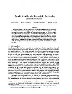
Before describing the parallel algorithm, we define what is meant by sweeping the flux across an unstructured grid to efficiently solve the Boltzmann equation for a particular ordinate direction. Consider the unstructured grid shown at the left of Fig. 1. Radiation propagates in the direction of the arrow at the upper left of the mesh. ~Note: This discussion is illustrated with a 2-D grid, but 3-D grids are conceptually identical.! Each grid cell in the mesh has one or more of its faces with normal vectors pointing in an “upwind” direction relative to the radiation direction. Similarly, each grid cell has one or more “downwind” faces. The computation of flux passing through a grid cell requires that we first know the flux entering the cell through its upwind faces. The flux attenuation can then be computed as it crosses the cell. The result is the flux exiting the cell through its downwind faces. This is the basic structure of the computational kernel in two discretization schemes for the Boltzmann transport equation on unstructured grids: the upwind corner balance ~UCB! method of Castrianni and Adams 12 and the discontinuous finite element method of Wareing et al.13 This description implies that the computation for a particular grid cell cannot be performed until the computations for cells that border it in an upwind sense are completed. Applied to the entire mesh, this means there are constraints on the order in which the grid cell computations are performed. Conceptually, this ordering is a sweep across the mesh starting from the upwind corner ~upper left of Fig. 1! toward the downwind corner ~lower right!. Formally, the order dependencies can be represented as a directed graph where each vertex is a grid cell and an edge is a face between two adjacent grid

Fig. 1. A 2-D unstructured finite element mesh and an associated directed graph. NUCLEAR SCIENCE AND ENGINEERING

VOL. 150

JULY 2005

269

270

PLIMPTON et al.

cells. A direction is assigned to each edge from the upwind vertex ~grid cell! to the downwind, as in the directed graph on the right side of Fig. 1. Equivalently, the graph also corresponds to a sparse matrix form of the Boltzmann equation, where the matrix is of order N ~number of grid cells or vertices! and a nonzero in matrix location ~ j, i ! represents an edge from vertex i to j in the directed graph. An ordering of the grid cells, which satisfies all geometric dependencies in the mesh and thus enables a successful sweep, is a topological sort of the vertices in the directed graph. If the graph is acyclic ~cycles are loops in the directed graph, a special case we return to in Sec. V!, then such an ordering is also a re-ordering of the rows of the sparse matrix so as to make it lower triangular. Solving the Boltzmann equation for a given ordinate direction on the grid is thus equivalent to traversing the directed graph and to solving a lower-triangular matrix equation. The latter can be done optimally via a direct method ~i.e., the sweep!; there is no need for an iterative solution. Now, consider the full transport problem with multiple energy groups and angles. The equations for different energy groups ~within a single angle! differ numerically but are represented by the same directed graph and matrix structure. However, different angles induce different ordering constraints, which flip the direction of some edges in the corresponding graph. Thus, each ordinate direction has its own directed graph and pattern of nonzeroes in its associated matrix. The parallel version of the full Boltzmann problem is to perform M sweeps ~or graph traversals or matrix solves! simultaneously on a set of grid cells that are distributed across processors, where M is the number of ordinate directions. A basic parallel algorithm for this problem 5,10,11 is given in Fig. 2 as a pseudocode that is executed by each processor. It is a modification of the obvious serial algorithm one uses to traverse a directed graph, extended to the case where the vertices of the graph are distributed across processors. The parallel algorithm has the advantage that graph orderings are never explicitly formed ~i.e., matrices are never stored!, either globally or within a processor’s subdomain. Rather, a simple counter is used to identify when all upwind dependencies of a grid cell in a particular ordinate direction are satisfied. Grid cells for which the flux can be computed ~the counter has become zero! are stored in a task list. By task, we mean the flux computation performed for all energy groups associated with a particular grid cell and a single ordinate direction. Before the algorithm begins, we assume the geometric and connectivity information for the finite element mesh has been distributed across processors in the usual way. A grid partitioner has been used to assign each processor some fraction of the grid cells, typically a compact subdomain of the grid. In a distributed-memory sense, we assume processors have no global knowledge of the

Fig. 2. Parallel algorithm executed by each processor for solving the Boltzmann equation on a distributed, unstructured grid for one or more ordinate directions.

grid; a processor stores information for grid cells only in its subdomain and the connections its grid cells make to neighboring grid cells owned by other processors. The algorithm begins with each processor precomputing the number of upwind faces each of its grid cells has for each ordinate ~angular! direction. Any cell0angle tasks with a count of zero are immediately added to the processor’s task list; these are grid cells at the upwind boundary of the global domain. Now, the processor enters a master loop that will continue until the flux is computed for all of its grid cells for all angles. The processor first loops over work on its task list. After all the energies associated with a cell0angle task are solved for, the counters for its downwind neighboring cells can be decremented. If the processor owns the downwind cell, it can decrement the counter directly. If the count goes to zero, the cell can be immediately added to the task list. If the downwind cell is owned by another processor, a small message must be sent to that processor, which identifies the cell0angle pair, the shared face, and the numeric flux values that propagate into the downwind cell. When the processor’s task list is empty, but it still has uncomputed work to do, this means it needs information from other processors to proceed. It either reads messages that have already arrived or waits for such a message. The data in the messages are used to decrement the counters for cells the processor owns, which then can potentially be added to the processor’s task list. This sequence of compute0send followed by receive is looped over until the processor has computed fluxes for all of its grid cells in all angular directions. Several comments concerning this basic algorithm are in order. First, the message passing is asynchronous in nature. Messages are sent whether the receiver is NUCLEAR SCIENCE AND ENGINEERING

VOL. 150

JULY 2005


waiting for them or not. All of the data exchanges in this algorithm can be implemented using the standard message-passing interface ~MPI! message-passing library 14 supported by all parallel machines, with calls to MPI_Send, MPI_Iprobe ~to check for incoming messages!, and MPI_Recv. In principle, MPI_Send is a blocking ~synchronous! call, but in practice for the tiny messages we are sending, it is nonblocking; the receiver queues the short messages. MPI_Recv is also blocking but is called only when a message is known to have arrived. A key feature of the algorithm is that the sweeps for multiple angles and energies can be computed simultaneously. A processor simply works on whatever task ~cell0 angle! is next on its list. So long as information about the relevant angle is encoded in the messages that processors send and receive, a processor can work on all the energies associated with a grid cell0angle pair as soon as the dependencies for that angle are satisfied. This is important because it avoids the long delay times that would arise if the flux associated with a single direction were being solved for across the entire grid before starting on another direction. In this scenario, a processor that owned grid cells far downwind would have to wait for all the upwind processors to finish before it could begin computing. The resulting idle time would seriously degrade parallel performance. In our implementation of this algorithm, we typically compute on all ordinate directions simultaneously to keep idle time to a minimum. We also note that this algorithm makes no assumptions as to how the unstructured grid is partitioned across processors. So long as the global graph associated with each angle is acyclic, this algorithm is guaranteed to eventually complete no matter which grid cells each processor owns. Even in the case of an ordinate direction tangential to the boundary between two processors so that flux values must potentially pass back and forth between the processors many times to perform the sweep, the algorithm will complete, albeit at the cost of many messages. We return to the question of computing an optimal grid partitioning in Sec. III. Finally, there are several enhancements one can make to this basic algorithm that we have omitted for purposes of simplicity. For example, on a machine with a high latency cost for initiating a send or receive, flux information for several grid cells can be buffered so as to send fewer, larger messages to neighboring processors. Incoming messages can also be probed for in the middle of the compute0send loop since incoming data may be more advantageous to compute on than the cell0angle pairs currently in the task list. We address this issue of task prioritization in Sec. III. The basic algorithm of Fig. 2 has been implemented in a parallel radiation solver package for finite element grids called SnRad, developed by the authors. The code computes flux solutions within a grid cell using the UCB discretization scheme of Castrianni and Adams.12 UCB NUCLEAR SCIENCE AND ENGINEERING

VOL. 150

JULY 2005

271

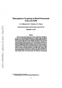
can be formulated for arbitrary finite elements such as tetrahedra, hexes, prisms, etc., and is particularly well suited for physical problems with sharp discontinuities in material properties, i.e., at interfaces. The package is used at Sandia National Laboratories ~SNL! in fluiddynamic and shock hydrodynamic simulation models of fires 15 and pulsed-power devices where target materials interact with X-rays.16 SnRad is a distributed-memory parallel code; it is written in standard C with calls to the MPI library for message passing. Figure 3 shows the performance of SnRad on a 3-D unstructured grid with 6360 hexahedral elements and 160 unknowns per element ~two energy groups, S8 quadrature with 80 ordinate directions!. The grid was created by meshing a rectangular box with parameters set so as to induce the meshing program to construct a nonuniform unstructured grid. With a million total unknowns, this is a large single-processor problem. For runs on P processors, the grid was partitioned into P subdomains using Chaco,17 discussed more fully in Sec. III. The parallel efficiency of SnRad running this fixed-size problem is plotted as a function of P for two machines at SNL. The Intel Tflops ~ASCI Red! is a traditional massively parallel supercomputer built with 333-MHz Pentiums. The CPlant machine is a commodity cluster built with 500-MHz DEC-Alpha processors. The Tflops machine has fast proprietary message-passing hardware ~310 megabytes0s bandwidth, 15-ms latencies for user-level MPI calls!; CPlant has a slower commercial Myrinet interconnect ~100 megabytes0s, 65 ms!. Anomalies in the timing data ~e.g., Tflops efficiency on eight processors!

Fig. 3. Parallel efficiency of the basic radiation sweep algorithm run on two different parallel machines, the Intel Tflops ~circles! and DEC-Alpha CPlant ~squares!. The benchmark problem used a fixed-size unstructured grid with 6360 hexahedral elements, an S8 quadrature, and two energy groups. The ideal curve ~triangles! is an estimated efficiency for this algorithm running on a hypothetical machine with infinitely fast communication.

272

PLIMPTON et al.

in this and later graphs may be due to variations in the shape of the irregular grid partitionings provided by Chaco since these can change dramatically when different numbers of processors are used. This does not, however, explain why the anomalies are not consistent between the two machines. This problem was first run on a single processor of each machine; the CPlant Alpha was roughly twice as fast as the Intel Pentium. The single-processor “grind time” ~CPU time0grid cell0angle0energy group! for the SnRad implementation of UCB for hex elements ~eight corner points! was 200 ms on the Pentium and 109 ms on the Alpha. As will be discussed in Sec. IV, the grind time is a strong function of the number of energy groups due to reuse of geometric calculations and cache effects in the innermost loop of the computational kernel. For larger numbers of energy groups, the grind time drops considerably. The performance data in Fig. 3 are not absolute run times but are parallel efficiencies normalized by the oneprocessor run time for each machine ~assumed to be 100% efficient!. For example, the 60% efficiency data point on 256 processors of the Tflops machine represents a run time 0.6{256 ⫽ 154 times faster than the one-processor Pentium run time. For this modest fixed-size grid, the scalability of the algorithm degrades as the processor count grows larger than a few dozen. This is particularly true on the CPlant machine because of its faster CPUs and slower communication ~particularly the high latency costs!. This is because the algorithm of Fig. 2 inherently requires a large number of small messages to be sent and received. Buffering data so as to send fewer, larger messages diminish the latency overhead but have the detrimental effect of making neighboring processors wait for information they could otherwise be computing with. This typically degraded performance; thus, in this benchmark small messages were sent as soon as offprocessor information was generated. The efficiency data of Fig. 3 lead to a natural question. How much of the inefficiency is due to the cost of data communication on a particular parallel machine and how much is due to one or more processors waiting for data to be computed ~and sent! by other processors before they can proceed with further computation? Note that no matter how fast interprocessor communication is, processors whose subdomain is in the center of the global grid will have to wait for sweep information to be computed and propagate inward from the outer boundaries. This will contribute to the inefficiency seen in Fig. 3. An idea suggested to us by Pautz 18 enabled us to distinguish between these two effects; Pautz discusses his use of this idea in his radiation solver in Ref. 10. For diagnostic purposes an option was added to SnRad to force the sweep algorithm to run in a synchronous fashion. Each processor computes a single task ~if it has one to work on! and then sends and receives any messages that result. An MPI_Barrier command is then

called to ensure that all messages arrive and are read by all processors before proceeding. All processors then advance forward one “clock tick” and repeat the same operations. The resulting code runs slowly because of the overhead of the many barriers, but the final count of how many clock ticks elapse before all processors finish their work enables an accurate measure of idle versus busy time. The parallel efficiency of the computation is equal to the total compute tasks divided by the quantity ~P times clock ticks!. It is a measure of how scalable the parallel sweep algorithm would be if message passing were infinitely fast with zero latency cost. It also provides an upper bound on the scalability we can expect to observe in an actual run. We call this the ideal efficiency; it is plotted as the curve of triangles in Fig. 3 for the 6360-element benchmark. The inefficiency in the Tflops and CPlant data is now broken into two pieces. The gap between the ideal curve and 100% efficiency is scheduling inefficiency inherent to the sweep algorithm as tasks are executed in a particular order by individual processors for a given partitioning of the global mesh. The gap between the ideal curve and the actual observed efficiency ~triangles, squares! is primarily communication inefficiency due to time spent sending and receiving data on a particular machine ~latency and bandwidth costs!. These costs are higher on CPlant than on Tflops because of the slower communication network. The ideal0actual gap also includes inefficiency due to small portions of SnRad that are inherently serial and do not fully parallelize. In Sec. III we discuss enhancements to the basic sweep algorithm that can reduce the scheduling inefficiency and thus shift the ideal and actual efficiency curves upward, yielding better overall performance.

III. ENHANCEMENTS

In this section we outline two improvements to the basic parallel sweeping algorithm of the previous section: a simple geometric heuristic for prioritizing the cell0 angle tasks each processor works on and a partitioning algorithm that can reduce the time processors must wait for other processors’ computations to satisfy data dependencies for their cell0angle tasks. In the basic algorithm of Fig. 2, ready-to-compute tasks were stored in a simple last-in, first-out stack where the most recently added task is the first to be computed on. More generally, the stack can be replaced with a priority queue, where each cell0angle task is assigned a numeric priority when added to the queue. When a task is requested from the queue, the highest-priority task is returned. In practice, a priority queue is implemented as a heap; adding a task or finding the highest-priority task are both inexpensive O~log~k!! operations, where k is the number of tasks in the heap at any one time. Since k NUCLEAR SCIENCE AND ENGINEERING

VOL. 150

JULY 2005


is typically small in the algorithm of Fig. 2, the overhead cost of using a priority queue versus a simple stack is negligible. Many different prioritization schemes can be used for sweeping algorithms on distributed unstructured grids. As discussed in Refs. 10 and 19, choosing an optimal prioritization scheme for a grid distributed across multiple processors can be recast in the most general sense as a graph-based scheduling problem that is known to be NP-complete ~not solvable by any algorithm whose cost is polynomial in N, where N is a function of the number of cell0angle tasks and processors, a very large number!. Pautz presents several graph-based heuristic solutions to this problem, based on analyzing the properties of the global directed graph associated with all ordinate directions. By contrast, we have implemented easier-to-compute geometric schemes that do not require graph-based information but exploit information about the single grid cell and ordinate associated with a task. The motivating idea is simple: Given a choice, a processor should preferentially work on a cell that imposes the most dependencies on other cells and other processors. Thus, a grid cell that is farther upwind should have higher priority. Numerically, for a particular cell0angle task, this value is computed as the negative of the dot product between the cell’s 3-D centroid position ~relative to the global mesh center point! and the vector for the ordinate direction. To avoid waiting, we also want a processor to work continuously on a single ordinate direction ~if tasks are available! so that useful information is passed as quickly as possible to nearby processors. We combine these two goals into a single priority value by multiplying the ordinate index by a large number and adding the smaller dot-product value to it. We call this a 3-D prioritization scheme. As will be shown below, this strategy boosts the ideal and actual efficiencies of the SnRad code by ;10% for large processor counts. Another distinction between our implementation and that of Pautz 10 is in how priority values are used to perform sweeps. Pautz precomputes a static schedule for each processor, which is then rigidly adhered to; each processor computes its tasks and communicates the results in a fixed sequence. We allow deviations from the schedule by dynamically selecting the highest-priority task that is currently available. This allows work to be done even when communication has delayed incoming tasks, but it may lead to a different task ordering that diverges from a static schedule that was otherwise superior. Note that both the graph- and geometry-based priority values must be recomputed if the grid geometry changes because of grid movement or adaptation. For the graph-based heuristics, this requires the ordinate graphs be traversed before performing sweeps; for our geometry-based approach, no precomputation is needed. Rather, we compute each priority on the fly, at the time a task is added to the priority queue. NUCLEAR SCIENCE AND ENGINEERING

VOL. 150

JULY 2005

273

We next address the question of how an unstructured grid should be partitioned across processors so as to minimize processor idle time as sweeps take place. The KBA algorithm 8,9 answered this question for structured grids: A 2-D columnar decomposition of the grid enables efficient sweeping across a 3-D structured grid, as shown in Fig. 4. Each of the nine processors in Fig. 4 owns a cluster of vertical columns of grid cells. For the ordinate direction shown by the large arrow, the front left processor must begin working before the others can. In the KBA algorithm, it works on its uppermost plane of grid cells ~fine grid! and then quickly passes needed information to its two neighboring processors so they can begin work. Soon each of the nine processors is working down its column as it receives flux information from its two upwind neighbors. This strategy pipelines the work for a single sweep, keeping all the processors busy. The first processor begins work on a new ordinate as soon as it finishes its work on a previous ordinate, keeping the pipeline filled as it loops over all ordinate directions within a single quadrant. It has been an open question whether a 2-D columnarstyle partitioning would yield similar benefits for sweeps on unstructured grids. Note that standard partitioning algorithms for 3-D unstructured grids assign equal numbers of grid cells to each processor while attempting to minimize the total number of cell faces that lie on the boundary between two processors. Tools like Chaco 17 and METIS 20 use graph-based algorithms such as spectral bisectioning or multilevel Kernighan-Lin for this purpose. The subdomains assigned to each processor are typically compact 3-D subsections of the global grid; this minimizes the surface-to-volume ratio of each subdomain. These algorithms are the methods of choice for unstructured grid partitioning in a variety of finite element applications since they minimize interprocessor communication. An example of this style of partitioning is shown on the left of Fig. 5 for a spherical domain

Fig. 4. A 2-D columnar decomposition of a 3-D structured grid as used by the KBA sweeping algorithm.

274

PLIMPTON et al.

Fig. 5. Partitioning of a gridded spherical domain with a 3-D spatial decomposition algorithm ~left! and a KBA-style 2-D columnar decomposition. Each processor’s subdomain is shown in a different shading; boundaries between processors are shown as thick lines.

meshed with an unstructured grid. Subdomains assigned to different processors are shown in different shades of gray; the thick black lines are the borders between processors. We call this a 3-D decomposition strategy; it was the algorithm used in Chaco to partition the 6360element grid for the benchmark results of Fig. 3. We added an option to Chaco to enable 2-D columnar partitioning of unstructured grids. An example is shown on the right of Fig. 5. This partitioning was computed in the following way, as illustrated in Fig. 6: The centroid point of each grid cell was first computed. Each 3-D point was then projected along a chosen ~KBA! axis into a 2-D plane normal to the axis. The resulting set of

Fig. 6. Projection of the centroid points of the cells of a 3-D unstructured grid into a 2-D plane. The 2-D points are partitioned geometrically using inertial cuts ~at levels A, B, and C! to generate a 2-D columnar decomposition of the original 3-D grid.

2-D points was then partitioned geometrically using an inertial method as shown by the lines in Fig. 6. The inertial method 21 computes the moments of inertia of a set of points, finding the axis around which the set of points has the smallest total inertia. The set of points is then split by a plane perpendicular to this axis, which is positioned so as to bisect the set of points. This procedure is applied recursively to each half of the partition, resulting in P equal-sized subsets of points for P processors. In Fig. 6, the first inertial cut on the 2-D set of points is labeled A, the second-level cuts are labeled with Bs, and the final level of cuts is labeled with Cs for this eight-processor example. Advantages of geometric partitioners such as the inertial method are that they are very inexpensive to compute and easily parallelizable.22 The Chaco package 17 has several geometric and graphbased partitioning options; this 2-D projection method was simple to implement as a modified Chaco option. When the partitioning of the 2-D projected points is mapped back to the original 3-D grid cells, the resulting subdomain shapes are roughly columnar ~with ragged boundaries!, as on the right of Fig. 5. We call this a KBA-style partitioning. When using it within SnRad, we alter the 3-D prioritization scheme described previously in the following way: Since we want the sweep to proceed down the columnar ~KBA! axis, we assign high priorities to cell0angle tasks at the top of the KBA columns. This is done by taking a dot product of the 3-D cell centroid with the KBA column direction and setting the sign of the dot-product value depending on the ordinate direction ~since which end of the column is the upwind end depends on the ordinate!. This quantity is then added to the ordinate index ~multiplied by a large number! in the same way as before. As with the 3-D prioritization scheme, this KBA-priority formula can be quickly computed on the fly using only geometric information NUCLEAR SCIENCE AND ENGINEERING

VOL. 150

JULY 2005


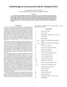
for a single grid cell; it does not require any global information or a traversal of the dependency graph. The 3-D and KBA prioritization schemes are implemented as options in our SnRad transport solver. ~The corresponding partitioning options are performed by Chaco as a preprocessing step.! The effects of these enhancements on the efficiency of the basic parallel sweeping algorithm are shown in Fig. 7. As before, a 3-D rectangular domain was gridded irregularly, this time with parameter settings that yielded a hexahedral grid with 25 032 elements. Again, an S8 quadrature with two energy groups was modeled, for a total of 4 million unknowns ~32 million corner points!. This problem was too large to fit on fewer than four processors of the Intel Tflops machine. One-processor timings ~100% efficiency! were accurately estimated from the computational grind times measured for hexahedral grid cells. On the left of Fig. 7, three ideal efficiency curves ~open symbols! are shown using the synchronized SnRad option described in Sec. II; note that the y axis in Fig. 7 begins at 50% efficiency. The lower curve of squares is the basic sweep algorithm of Sec. II and a traditional 3-D partitioning of the grid. The middle curve of triangles is for runs using the same partitioning with the 3-D prioritization scheme described above. The upper curve of circles is for runs using the KBA-style partitioning and prioritization. Each enhancement offers an ;10% improvement in ideal efficiency on large numbers of processors. Their effect on actual run-time performance is shown on the right of Fig. 7, using corresponding shaded symbols. As in Fig. 3, actual per-

Fig. 7. Parallel scalability of the basic sweeping algorithm ~squares!, the 3-D prioritization scheme with a 3-D partitioning ~triangles!, and the KBA prioritization scheme with a KBA-style 2-D columnar partitioning ~circles!. Ideal efficiencies are on the left; actual run-time efficiencies are on the right for the Intel Tflops machine. An irregular grid on a 3-D rectangular domain was used with 25032 hexahedral elements, with an S8 quadrature ~80 ordinates! and two energy groups. NUCLEAR SCIENCE AND ENGINEERING

VOL. 150

JULY 2005

275

formance never exceeds the predicted ideal performance, but a similar 5 to 10% improvement between the basic and enhanced algorithms is evident.

IV. PERFORMANCE RESULTS

The algorithms of Secs. II and III were benchmarked using SnRad on a series of unstructured hexahedral meshes of various sizes on the Intel Tflops machine. In Fig. 8 we show parallel efficiencies for the block-shaped domain discussed in Sec. II, meshed at three different resolutions. The grid sizes were 6360, 25 032, and 99 702 elements. All the benchmarks were run with an S8 quadrature ~80 ordinate directions! and two energy groups, yielding a total number of unknowns of approximately 1 million, 4 million, and 16 million for the three problems. Efficiency curves are plotted for each fixedsize problem running on various numbers of processors. The larger problems cannot fit on a single processor; as

Fig. 8. Fixed-size parallel efficiency of the SnRad radiation solver on the Intel Tflops machine for a block-shaped domain meshed with an unstructured grid at three different resolutions. N is the total number of unknowns as discussed in the text. As in Fig. 7, the shaded circles are actual efficiencies for the sweep algorithm with a KBA-style decomposition and prioritization scheme, the open circles are the associated ideal efficiencies, and the shaded squares are the actual efficiencies for the basic algorithm with a 3-D decomposition and no prioritization.

276

PLIMPTON et al.

before, the 100% efficiency one-processor timings for these cases were estimated from the measured grind times. For each grid size, three curves are plotted. The top curve ~open circles! is the ideal efficiency using a KBAstyle decomposition of the unstructured grid with the associated prioritization scheme discussed in Sec. III. The middle curve ~shaded circles! is the actual run-time efficiency for the same case. The lower curve ~shaded squares! is the actual efficiency for the basic algorithm of Sec. II using a 3-D decomposition and no prioritization. The same trends observed in Sec. III are evident here. The largest problem gets an ;20% boost in actual efficiency because of the two enhancements, with an overall efficiency of .80% on 256 processors ~a speedup of .200 times versus the estimated one-processor timing!. In Fig. 9, we plot efficiency curves for the spherical problem described in Sec. III, gridded at four different resolutions. These problems were also run with S8 and two energy groups. The grid sizes used were much larger ~approximately 108 000, 500 000, 1 048 000, and 3 322 000 elements each! and were run on up to 2048 processors of the Tflops machine. In the largest problem more than 500 million unknowns, or more than 4 billion corner values in the UCB formalism, are being solved for during each sweep.

Fig. 9. Fixed-size parallel efficiency of SnRad on the Tflops machine for a spherical geometry meshed with an unstructured grid at four different resolutions. The meanings of N ~total unknowns! and the curve symbols are the same as in Fig. 8.

The labeling ~open and shaded circles, shaded squares! within each set of three curves is the same as before. The data indicate some degradation in efficiency, both ideal and actual, on thousands of processors, which is probably due to the high communication load that a radiation transport sweep incurs, even on a well-balanced parallel machine like the Intel Tflops. The largest problems are running at a little more than 60% efficiency on 2048 processors, which is a reasonable aggregate performance for a fixed-size problem. We note that on all but the largest problem the runtime difference between the basic and enhanced algorithms is slowly shrinking as the number of processors increases. This could be due to increased communication costs for the KBA decomposition on very large numbers of processors; the partitions become longer and narrower with higher surface0volume ratios. We also note that on the largest number of processors, all of the problems have roughly equal efficiency ~60 to 65%!, independent of problem size. Since the ideal efficiency in these cases also peaks at ;70%, this may indicate a fundamental limitation with all these sweeping algorithms for thousands of processors. Even with a KBAstyle decomposition, some of the 2048 processors will be surrounded by many other processors’ subdomains and have little work to do ~at the top and bottom of their subdomain! before having to wait for flux information from processors on the periphery of the global domain. In Fig. 10, we benchmark the performance of our algorithms in SnRad as the number of ordinates is varied. A spherical geometry was used, gridded with 32 000 hexahedral elements. The benchmark was run with two energy groups on 256 processors of the Intel Tflops.

Fig. 10. Parallel efficiency of SnRad on 256 processors of the Tflops machine for varying numbers of ordinate directions. A spherical geometry meshed with an unstructured grid of 32 000 elements was used. Both ideal and actual efficiencies are shown for the basic algorithm ~squares! and the 3-D and KBA-enhanced versions ~triangles and circles!. NUCLEAR SCIENCE AND ENGINEERING

VOL. 150

JULY 2005


Ordinate quadratures from n ⫽ 2 to n ⫽ 20 ~8 to 440 angular directions! were used; the total number of unknowns varied from 512 000 to just more than 28 million. On the left of Fig. 10, three ideal efficiency curves are plotted, for the basic algorithm ~squares!, the 3-D prioritization ~triangles!, and the KBA decomposition with a KBA-style prioritization ~circles!. The corresponding actual run-time efficiencies are plotted on the right side of Fig. 10 in shaded symbols. Clearly, all the algorithms suffer from reduced efficiency for low-order quadratures. This is because the wait times for some processors to begin working are a larger fraction of the total run time when there is less computation to perform. As in previous plots, the actual efficiencies in Fig. 10 track the ideal efficiencies fairly closely; the ideal values impose an upper bound for all the data points shown. One interesting attribute of the actual run-time data for the two enhanced algorithms ~triangles, circles!, is a crossover in performance that occurs at about S12 ~168 ordinates!. For large numbers of ordinates, the 3-D decomposition and its associated prioritization scheme become more efficient than the KBA decomposition, by ;10%. This again could be due to the increased communication costs that the KBA decomposition, with its long narrow subdomains, requires relative to more traditional 3-D partitionings. Finally, in Table I we show the effect of the number of energy groups on single-processor performance and parallel scalability in SnRad. The 3-D rectangular domain of Sec. II and Fig. 8 was gridded with 6360 hexahedral elements and benchmarked on 256 processors of the Intel Tflops with an S8 quadrature ~80 ordinates! using the basic sweep algorithm of Sec. II. The number of energy groups was varied from 1 to 256 ~508 800 to 130 million unknowns!, yielding the parallel run times for each sweep as shown in Table I. The one-processor time for these runs was estimated by the fraction of the parallel run time spent in computation and converted to a grind time ~microseconds per grid cell per ordinate per energy group!. The estimated one-processor time was then compared to the actual sweep time to compute the

277

efficiency of the 256-processor parallel runs, as listed in Table I. The data indicate that for small numbers of energy groups, there is almost no additional computational cost ~per sweep! to adding extra groups. This is due to two effects mentioned briefly in Sec. I. The flux values for different energy groups are stored contiguously in SnRad data structures for a particular grid-cell0angle pairing. Since the computations for different energy groups are also done in the innermost loop within an SnRad solve, this has a favorable cache effect. The relatively expensive grid geometry operations that SnRad performs as a sweep progresses ~face normals and areas, corner orderings! do not need to be repeated for additional energy groups, giving an additional savings. A further optimization we do not currently exploit in SnRad would be to precompute some or all of these grid geometry factors. This would require additional storage, and the factors would also need to be recomputed on any time steps where the grid deformed. The latter is a common occurrence in the shock-hydrodynamics applications, where Lagrangian grids are employed. We note that computing fluxes for multiple ~or all! energy groups simultaneously in a single ordinate sweep may be detrimental to the convergence rate of the overall source iteration. For example, in neutronics problems with significant downscattering, it is often advantageous to perform complete sweeps in sequence from high to low energy. SnRad allows the user to specify how many energy groups to work on simultaneously so these tradeoffs can be explored. The reason that the parallel efficiencies in Table I fall off as energy groups increase is that the message passing in our algorithm incurs a fractionally greater cost. For low group counts, the communication cost is latency dominated; message sizes are small. For high group counts, a significant amount of data must be exchanged, and additional bandwidth costs result. For 256 energy groups, the data for the face of a single grid cell is 8192 bytes ~four corner points, 256 groups, double precision flux values!, which is the minimum size of a data packet

TABLE I Grind Times ~Per Grid Cell! and Parallel Efficiencies as a Function of Number of Energy Groups for a Rectangular Domain Gridded with 6360 Hexahedral Finite Elements on 256 Processors of the Intel Tflops Energy Groups

Sweep time ~s! Grind time ~ ms! Parallel efficiency ~%!

1

2

4

8

16

32

64

128

256

1.27 398 62.4

1.31 200 61.0

1.31 102 61.9

1.40 52.8 60.1

1.61 28.3 55.8

2.05 16.3 50.6

3.04 10.8 45.3

5.14 8.37 41.4

10.0 7.09 36.1

NUCLEAR SCIENCE AND ENGINEERING

VOL. 150

JULY 2005

278

PLIMPTON et al.

that must be sent to an adjacent processor.a At 310 megabytes0s ~interprocessor bandwidth on Tflops!, this requires ;25 ms to send0receive, compared with the latency-only cost on Tflops of 15 ms. This additional bandwidth cost accounts for the drop in efficiency of a factor of ;2 from 60 to 35% as energy groups go from 1 to 256 in Table I. The results of this section indicate that overall performance and scalability are a complex function of grid size, number of ordinates and energy groups, number of processors, and choice of grid decomposition and prioritization. The unstructured grids we have used as benchmarks are prototypical ~rectangular and spherical global domains!, but results on application-specific grids might also vary somewhat. Finally, parallel machines with differing communication characteristics can also differ in performance, as in Fig. 3. Our conclusion is that the KBA-style decomposition and prioritization scheme we have outlined are generally the fastest choices. However, their advantages are sometimes not more than a few percent over the basic parallel sweep algorithm or other decompositions and are subject to the issues of the previous paragraph. Thus, it is useful to have algorithmic options within a discrete ordinates solver package, for grouping of sweeps by energy and angle, for grid decomposition, and for prioritization schemes. This allows users to perform their own benchmark testing for a particular problem’s physics and geometry characteristics, grid size, and choice of parallel machine and number of processors.

V. CYCLE DETECTION AND ELIMINATION

The preceding discussion ignored one issue with sweeping algorithms that is important to address for unstructured grids: what to do if one or more cycles exist in the directed graph associated with any of the ordinate directions. A cycle is a loop in a directed graph, as at the left of Fig. 11. In the radiation transport context, cycles can occur in the dependency graphs associated with large, complex tetrahedral or hexahedral finite element meshes. They occur quite commonly if a Lagrangian mesh is twisted or deformed because of material response. Note that if the simulation grid never changes during a simulation, identifying cycles can be done as a serial preprocessing step, though it can be an expensive computation for large grids and high-order quadratures. However, if the grid geometry changes because of deformation or adaptation, finding cycles in parallel is a necessity. The sketch at the right of Fig. 11 is a simple example of a cycle. Imagine a circular ring of hexahedral elea Large

messages may cause the send operations in the algorithm of Fig. 2 to block in some MPI implementations. This can typically be overcome by user-defineable MPI settings that allow for large nonblocking sends.

Fig. 11. A directed graph with a cycle ~left! and a twisted ring of mesh elements that induces a cycle.

ments whose top surface is twisted slightly relative to the lower surface. A radiation direction down the ring axis will create a cycle in the associated graph. The problem that cycles cause for the algorithm of Fig. 2 is that the computation for one or more elements cannot be performed because their upwind dependencies will never be satisfied; a grid cell depends on itself. In parallel, the sweep algorithm will “hang” as a processor waits for a message that will never be sent. In matrix terms, a cycle means there is no ordering of elements that creates a lower triangular matrix equation; it is impossible to solve in a single sweep. In serial, the solution to this problem is typically to “break” the cycle by removing one or more edges of the dependency graph, which is equivalent to zeroing matrix elements in the upper-triangular portion of the associated matrix equation. Old radiation flux values ~from a previous source iteration or a previous time step! are used for this face, and the sweep is performed as before. The physical justification is that one ~or more! of the element faces that make up the cycle will likely be oriented obliquely with respect to the ordinate direction. Since very little flux passes through that face, using old values for its contribution to the solution should have a negligible effect on the convergence rate of the overall source iteration. In graph terminology, the strongly connected components ~SCCs! within each ordinate’s dependency graph must be identified. An SCC is a set of vertices in a directed graph, any of which are reachable from all the others. An SCC may contain multiple cycles; consider a figure-eight–shaped SCC where the center vertex is part of two cycles. The best serial algorithm for finding SCCs is due to Tarjan.23 It requires time that is linear in the number of graph edges and relies on depth-first traversal ~DFT! of the graph. Unfortunately, DFTs do not parallelize well for distributed graphs. This is because a DFT is performed by walking from grid cell to grid cell across the entire grid, which is an inherently serial operation. By contrast, the sweeping algorithm of Fig. 2 operates in an order more akin to a breadth-first traversal ~BFT! of NUCLEAR SCIENCE AND ENGINEERING

VOL. 150

JULY 2005


the graph. When the computation for one grid cell is performed, all of its downwind neighbors are ~potentially! added to the task queue. BFTs are more readily parallelizable than DFTs, as evidenced by the parallel efficiency results of Sec. IV. We have developed an alternative SCC-finding algorithm that is based on BFT-style operations and is thus more parallelizable than Tarjan’s algorithm. A detailed description of the algorithm and its complexity analysis is given in Refs. 24 and 25 from a computer-science perspective. Here, we provide a brief description of its basic ideas in the context of radiation transport sweeps and additional details about how it is used to both find and break cycles within our SnRad transport solver. We first describe how the new algorithm works for a single graph ~ordinate direction! and then outline the full parallel implementation for multiple ordinates. Imagine a finite element mesh with two cycles, shown as oval rings at the left of Fig. 12, and a directed graph associated with the ordinate direction given by the arrow at the upper left. Recall that in the sweep operation any elements whose upwind counters decrement to zero cannot be in a cycle ~or SCC!. This fact is exploited by first performing a downwind sweeplike operation called a trim, which identifies and discards elements that are not in an SCC. In parallel, the trim operates like the algorithm of Fig. 2 with two modifications. First, no flux or UCB computations are performed. The graph is simply traversed, counters decremented, messages sent and received, and grid cells flagged for deletion when their upwind dependencies are all satisfied. Second, if an SCC is present, the trim will not complete, and the parallel code must detect when this occurs ~and not hang!. Spe-

Fig. 12. A finite element mesh ~2-D blob! containing two cycles shown as oval rings. The original mesh on the left is trimmed, leaving the shaded portion. On the right, the remaining portion is marked, which breaks the mesh into three partitions: upwind ~lines!, downwind ~checked!, and unreachable ~unshaded!. NUCLEAR SCIENCE AND ENGINEERING

VOL. 150

JULY 2005

279

cial termination-detection logic is added to the sweep algorithm to enable this. In addition to owning a portion of the finite element grid, each processor is also assigned a location within a binary tree containing all the processors. When a processor is waiting for an incoming trim message, it sends a special message to its parent in the tree, saying it is waiting. If the parent processor is also waiting, it looks for wait messages coming from both its children in the binary tree and then sends a wait message to its parent. The processor at the root of the tree reverses the direction of the message passing and sends a message to its children. These wait messages percolate up and down the tree of processors as the trim is proceeding. If a processor does further trim work before a wait message returns to it, it flags the wait message appropriately, and the up0down percolation continues. If the wait messages ever go completely up and down the tree without any processor doing additional trim work ~and if all sent messages have also been received!, then all processors are waiting because of an SCC, and they can exit the trim. For the mesh of Fig. 12, the upper SCC ~oval ring! will block the first downward trim so that grid cells in its “shadow” between the two open arrows are never reached. A second upwind trim is then performed, which will block at the second SCC, leaving grid cells between the shaded arrows. When all grid cells ~vertices! reached by both trim operations are deleted from the dependency graph, the shaded region remains; the six-sided polygon at the right of Fig. 12 represents this remaining portion of the original graph. A random pivot vertex ~black dot! is now selected within the remaining graph. A BFT-style mark operation is then performed, that flags vertices that are upwind and downwind of the pivot. In the mark operation, each vertex is flagged as upwind or downwind when it is reached, and its neighbors ~ancestors or descendants! can then be likewise marked, without all their dependencies being satisfied. As in the sweep, messages are sent to processors owning neighboring vertices ~grid cells! when appropriate. As in the trim, termination-detection is also implemented so that all processors know when the marking is complete. Note that unlike the sweep or trim, which only advances when all dependencies are satisfied, a mark operation does not block at an SCC but passes through it in both directions. After the marking is complete, some vertices may have been flagged as being both upwind and downwind from the pivot. If so, this set of vertices ~including the pivot! is precisely an SCC. The graph edges that make up the SCC are tested to find the corresponding cell face with the smallest projected surface area with respect to the ordinate direction. That edge is removed from the graph, which breaks at least one cycle in the SCC. Also note that the mark operation partitions the graph into four disjoint subgraphs: the vertices upwind from

280

PLIMPTON et al.

the pivot ~lined region at right of Fig. 12!, the vertices downwind ~checked region!, vertices that are neither ~unshaded region!, and the SCC itself ~minus the removed edge!. The key observation 24 that makes this algorithm work is that no SCC remaining in the graph can include vertices from more than one of these subgraphs. The overall algorithm ~trim, pick pivot, mark! can thus be invoked on each subgraph. The algorithm proceeds in a recursive fashion, breaking the graph into smaller and smaller pieces, detecting and eliminating cycles one by one whenever a pivot vertex is in an SCC. The recursive nature of this algorithm leads to an expected complexity of O~N log N ! ~Ref. 24!, compared with the linear-time complexity of the Tarjan algorithm. However, from a parallel perspective, this algorithm is more parallelizable than Tarjan’s because the trim and mark operations both involve breadth-first style graph traversals. Since dependency graphs for many ordinate directions must be searched for SCCs, the trim and mark operations can also be performed on multiple graphs simultaneously to achieve greater parallelism, as in the parallel sweep algorithm of Fig. 2. The parallel version of the algorithm is outlined in Fig. 13. It is invoked within SnRad initially and whenever the geometry of the finite element mesh changes ~via movement or adaptation!, since such changes alter the ordinate dependency graphs. The first step of the parallel-cycle–detection algorithm is to identify the set of graphs to search for SCCs. Sn quadratures typically include pairs of ordinates in opposite directions. The two graphs associated with such a pair have the same structure; their edge directions are simply the reverse of each other. Thus, only one graph from each pair need be searched for SCCs. A list of these

graphs is generated, with each processor owning the subpiece of each graph corresponding to its grid cells. The algorithm then enters its recursive phase. All the graphs are trimmed simultaneously ~in parallel!, first in the downwind direction ~which will completely eliminate any graphs that have no SCCs!; then, the remaining portions are trimmed in the upwind direction. A pivot vertex is chosen within each remaining portion; then, the portion is marked. The marking may identify an SCC in some of the graphs. An appropriate edge is eliminated from each SCC, and the edge ~cell face! information is stored so that the radiation solver can later eliminate the edge from the sweep graphs and use appropriately modified flux values in the UCB solution for the affected grid cell. For each marked graph, three new subgraphs are formed ~four if an SCC was found! using the sets of upwind, downwind, and unmarked vertices and their associated edges. At the end of each recursive stage, a new list of distributed graphs has been formed, and the old list is discarded. The new list is processed in the same fashion until all cycles in all of the graphs have been detected and eliminated. At this point there are no graphs left in the list, so the algorithm exits, returning a distributed data structure containing the information for broken edges ~face0ordinate pairings! on each processor. It is important to realize that each stage of the algorithm in Fig. 13 is synchronous and parallel in nature; all the processors work on all the graphs together and then move to the next stage of the algorithm. Initially, each processor owns a portion of every top-level graph. As the graphs are trimmed and partitioned, an individual graph may end up spanning only a subset of processors. But, even if a processor owns no vertices in any graph of the current list ~no cycles remain in its portion of the

Fig. 13. Parallel recursive algorithm for detecting and breaking cycles in the directed graphs associated with radiation transport in one or more ordinate directions on a distributed unstructured grid. NUCLEAR SCIENCE AND ENGINEERING

VOL. 150

JULY 2005


grid!, it still continues to step through the algorithm with the other processors until all are finished. The trim and mark steps within Fig. 13 are asynchronous operations similar to the sweep algorithm of Fig. 2. Other operations such as picking a pivot vertex or identifying the correct edge to remove require coordination between the processors that jointly own a particular subgraph. As with sweeping, the cycle-detection algorithm does not require any global graphs ever be assembled; simple counters for each cell0ordinate pair are used to flag upwind0downwind dependencies as graphs are traversed in the trim and mark operations using only the finite element connectivity information. Overall, the data structures needed for this algorithm require considerably less memory than the transport flux solution since the storage for energy groups and corner points is not needed. We have benchmarked the cycle-detection algorithm on two grids that enable cycles to be generated in a controlled fashion. The grid geometries are shown in Fig. 14. The first is a hollow cylinder where the grid is twisted by 10% along the cylinder axis. As in Fig. 11, this induces SCCs for ordinate directions close to the cylinder axis. The SCCs tend to be large and highly connected ~many cycles in a single SCC!. The second geometry is a cube where each grid point is displaced in a random direction by a random amount up to 30% of the distance between neighboring grid points. This induces many small SCCs because of the large deformation of individual grid cells. The performance of the cycle-detection algorithm within SnRad on these two benchmark geometries is shown in Fig. 15. For these timings entire SCCs were removed from an ordinate graph when found, rather than breaking single edges inside the SCCs and performing further recursion ~see discussion below!. An S20 quadrature was used with 440 ordinate directions or 220 unique dependency graphs. For both meshes the grid resolution was varied with the number of processors so as to keep the grid-cell0processor ratio constant at 1000. The cubic

Fig. 14. Two grids for testing cycle detection. Left: a hollow cylinder with the grid twisted along the vertical axis; right: a cube where each grid point is displaced by a small random amount. NUCLEAR SCIENCE AND ENGINEERING

VOL. 150

JULY 2005

281

Fig. 15. CPU run times for cycle detection within SnRad on the Tflops and CPlant machines for the two grid geometries of Fig. 14 using an S20 quadrature ~440 ordinates!. For both problems the mesh resolution was scaled with the processor count; all grids contain 1000 elements per processor.

geometry was meshed at a 10 ⫻ 10 ⫻ 10 resolution for one processor and at an 80 ⫻ 80 ⫻ 160 resolution for 1024 processors. In the cylindrical meshes, increasing resolution did not change the total number of 40 SCCs in all 220 graphs. In the cubic meshes, the number of SCCs increased rapidly with the grid size. On the smallest mesh of 1000 cells, there were 65 SCCs; on the largest mesh of 1 024 000 cells, there were 41 999 SCCs. Thus, from a parallel perspective these two problems are both scaledsize benchmarks in grid size, but the cylinder is a fixed-size benchmark in SCC count while the cube is a scaled-size benchmark in SCC count. The run times are plotted for varying numbers of processors on both the Intel Tflops ~circles! and DECAlpha CPlant ~squares! machines. For the twisted cylinder, perfect scalability would be a horizontal line on these scaled-size grids. The performance is reasonably scalable up to 64 processors on both machines and then increases to 12.8 s on 1024 processors of Tflops ~a parallel efficiency of 24.5%!. The inefficiency is due in part to load imbalance that occurs after trimming and recursion when some processors no longer own grid cells in the graphs that remain. It is more difficult to quantify what perfect scalability should be for the deformed cube grids since the number of SCCs rises dramatically with increasing processor count. This induces much deeper levels of recursion in the cycle-detection algorithm as longer and longer lists of graphs are generated. Each machine’s one-processor time for the deformed cube problem is about the same as its time on the twisted cylinder problem, but the run times rise to 45.1 and 159.6 s on 512 processors of the two machines. The more important metric is how the cost of cycle detection compares to the sweep times for a transport

282

PLIMPTON et al.

solution. For a grind time of 200 ms on the Tflops machine ~see Sec. II!, a 512 000 grid cell problem with 440 ordinates and two energy groups would give a sweep time of 176 s on 512 processors if the run were 100% parallel efficient. In this context, the 45.1-s cycledetection time is roughly the same expense as a single sweep in a source iteration solution ~requiring many sweeps! within a single time step. As mentioned, the timings of Fig. 15 were for finding SCCs but not breaking them. The breaking algorithm described above worked well for the deformed cube problem. Because its SCCs contain only a few grid cells on average, breaking a single minimum-flux edge typically eliminated the entire SCC on the next round of recursion. The overall run time with breaking enabled increased by only a few percent. However, for the twisted cylinder problem, single SCCs can contain hundreds or thousands of grid cells and similar numbers of cycles. Breaking edges one at a time is inefficient, causing the algorithm to recurse much more deeply and consume more memory. For example, the run time on eight Tflops processors increased from 3.83 to 51.6 s when breaking was enabled. The ideal solution to this problem would be to identify the minimal set of edges to break within an SCC that would eliminate all cycles. In graph nomenclature, this is the minimum arc feedback set, and unfortunately, finding it would be difficult in parallel and is an NP-complete problem in the number of edges in the SCC. A simpler heuristic would be to break multiple edges, perhaps all those with associated radiation flux below some threshold. We are still experimenting with practical solutions to the edge-breaking task in special cases such as this and the effect edge-breaking choices have on subsequent radiation sweeps.

VI. CONCLUSIONS

We have presented two parallel algorithms that address issues relevant to solving the Boltzmann transport equations via the method of discrete ordinates on unstructured grids. They are suitable for transport problems requiring large grids running on large parallel machines, where the grid must be distributed across processors. The algorithms allow the radiation equations to be solved with the same sweeping method that is often optimal for a serial implementation. The first algorithm performs full sweeps in multiple ordinate directions simultaneously. The second finds and eliminates cycles in all sweep dependency graphs, a necessary precursor to computing sweep solutions on unstructured grids. We have also described two enhancements to the sweep algorithm that improve its parallel efficiency. The first is an easily computed geometric formula that prioritizes a processor’s choice of which grid cell0ordinate task to work on. The second is a grid-

partitioning algorithm that enables unstructured grids to be decomposed across processors in a 2-D columnar fashion, similar to the structured grid partitions used effectively in the KBA sweeping algorithm. The two enhancements can be used separately or in tandem. For example, if the grid-partitioning strategy is constrained by other portions of the simulation ~e.g., by fluid or hydrodynamic solvers!, then using the prioritization idea by itself can improve parallel performance. The algorithms have been benchmarked on two large parallel machines for several finite element meshes with up to 3 million elements ~500 million radiation flux unknowns or 4 billion UCB corner point unknowns!. Parallel efficiencies on large numbers of processors ~up to 2048! were typically .50% for the basic sweep algorithm and up to 80% for the enhanced algorithm. We note that these results are for fixed-size problems, not scaled-size problems ~constant element0processor ratio! on which it is typically easier to achieve high efficiencies. Finally, we note that parallelizaton of a complete source iteration scheme requires that the acceleration method also be parallelized, not only the sweep operations. Since the transport synthetic acceleration method 4 performs sweeplike operations, it can potentially be parallelized by algorithmic ideas similar to those proposed here.

ACKNOWLEDGMENTS This work was performed at SNL, a multiprogram laboratory operated by Sandia Corporation, a Lockheed-Martin company, for the U.S. Department of Energy ~DOE! under contract DE-AC-94AL85000, and has been sponsored by DOE’s ASCI program. We have had many fruitful discussions and received helpful suggestions on this work from M. Adams of Texas A&M University; P. Nowak of LLNL; R. Baker and K. Budge of LANL; and S. Pautz, formerly at LANL, now at SNL. Pautz and Baker also provided constructive comments on this manuscript.

REFERENCES 1. P. BROWN, B. CHANG, F. GRAZIANI, and C. S. WOODWARD, “Implicit Solution of Large-Scale Radiation-Material Energy Transfer Problems,” Proc. 4th Int. Symp. Iterative Methods in Scientific Computation, Austin, Texas, October 18–20, 1998, IMACS Ser. Comput. Appl. Math., 5. 2. C. R. DRUMM, “ Parallel Finite Element Electron-Photon Transport Analysis on 2-D Unstructured Meshes,” SAND990098, Sandia National Laboratories ~1999!. 3. M. L. ADAMS and W. R. MARTIN, “Diffusion-Synthetic Acceleration of Discontinuous Finite-Element Transport Iterations,” Nucl. Sci. Eng., 111, 145 ~1992!. NUCLEAR SCIENCE AND ENGINEERING

VOL. 150

JULY 2005


283

4. G. L. RAMONÉ, M. L. ADAMS, and P. F. NOWAK, “Transport-Synthetic Acceleration Methods for Transport Iterations,” Nucl. Sci. Eng., 125, 257 ~1997!.

14. “MPICH Standard at Argonne National Laboratories”; available on the Internet at ^http:00www-unix.mcs.anl.gov0 mpi0index.html&.

5. S. PLIMPTON, B. HENDRICKSON, S. BURNS, and W. McLENDON III, “ Parallel Algorithms for Radiation Transport on Unstructured Grids,” Proc. SC2000 Conf., Dallas, Texas, November 4–10, 2000, Association for Computing Machinery0 Institute of Electrical and Electronics Engineers ~2000!.

15. S. P. BURNS, “Spatial Domain-Based Parallelism in LargeScale, Participating-Media, Radiative Transport Applications,” SAND96-2485, Sandia National Laboratories ~1996!.

6. Y. Y. AZMY, “Multiprocessing for Neutron Diffusion and Deterministic Transport Methods,” Prog. Nucl. Energy, 31, 317 ~1997!. 7. P. NOWAK and M. K. NEMANIC, “Radiation Transport Calculations on Unstructured Grids Using a Spatially Decomposed and Threaded Algorithm,” Proc. American Nuclear Society Conf. Mathematics and Computation, Reactor Physics and Environmental Analysis in Nuclear Applications, p. 379 ~1999!. 8. R. S. BAKER and R. E. ALCOUFFE, “ Parallel 3-D Sn Performance for DANTSYS0MPI on the Cray T3D,” Proc. Joint Int. Conf. Mathematical Methods and Supercomputing for Nuclear Applications, Saratoga Springs, New York, October 5–9, 1997, Vol. 1, p. 377, American Nuclear Society ~1997!. 9. R. S. BAKER and K. R. KOCH, “An Sn Algorithm for the Massively Parallel CM-200 Computer,” Nucl. Sci. Eng., 128, 312 ~1998!. 10. S. D. PAUTZ, “An Algorithm for Parallel Sn Sweeps on Unstructured Meshes,” Nucl. Sci. Eng., 140, 111 ~2002!. 11. Y. Y. AZMY and D. A. BARNETT, “Arbitrarly High Order Transport Method of the Characteristic Type for Tetrahedral Grids,” Proc. Int. Mtg. Mathematical Methods for Nuclear Applications, Salt Lake City, Utah, September 2001 ~2001! ~CD-ROM!. 12. C. L. CASTRIANNI and M. L. ADAMS, “A Nonlinear Corner Balance Spatial Discretization for Transport on Arbitrary Grids,” Nucl. Sci. Eng., 128, 278 ~1998!. 13. T. A. WAREING, J. M. McGHEE, J. E. MOREL, and S. D. PAUTZ, “Discontinuous Finite Element Sn Methods on ThreeDimensional Unstructured Grids,” Nucl. Sci. Eng., 138, 256 ~2001!.

NUCLEAR SCIENCE AND ENGINEERING

VOL. 150

JULY 2005

16. M. K. MATZEN, “Z Pinches as Intense X-Ray Sources for High-Energy Density Physics Applications,” Phys. Plasmas, 4, 1519 ~1997!. 17. B. HENDRICKSON and R. LELAND, “The Chaco User’s Guide: Version 2.0,” SAND94-2692, Sandia National Laboratories; available on the Internet at ^http:00www.cs. sandia.gov0;bahendr0chaco.html& ~1994!. 18. S. D. PAUTZ, Los Alamos National Laboratories, Personal Communication. 19. N. M. AMATO and P. AN, “Task Scheduling and Parallel Mesh-Sweeps in Transport Computations,” TR00-009, Department of Computer Science, Texas A&M University ~2000!. 20. G. KARYPIS and V. KUMAR, “A Fast and High Quality Multilevel Scheme for Partitioning Irregular Graphs,” CORR 95-035, University of Minnesota, Department of Computer Science; available on the Internet at ^http:00www-users. cs.umn.edu0;karypis0metis0index.html& ~1995!. 21. V. TAYLOR and B. NOUR-OMID, “A Study of the Factorization Fill-in for a Parallel Implementation of the Finite Element Method,” Int. J. Numer. Methods, 37, 3809 ~1994!. 22. B. HENDRICKSON and K. DEVINE, “Dynamic Load Balancing in Computational Mechanics,” Comput. Methods Appl. Mech. Eng., 184, 485 ~2000!. 23. R. E. TARJAN, “Depth First Search and Linear Graph Algorithms,” SIAM J. Comput., 1, 2, 146 ~1972!. 24. L. FLEISCHER, B. HENDRICKSON, and A. PINAR, “On Identifying Strongly Connected Components in Parallel,” Proc. Irregular’2000, Lecture Notes in Computer Science, SpringerVerlag ~2000!. 25. W. McLENDON III, B. HENDRICKSON, S. PLIMPTON, and L. RAUCHWERGER, “Identifying Strongly Connected Components in Parallel,” Proc. 10th SIAM Parallel Processing for Scientific Computing Conf., Portsmouth, Virginia, March 12–14, 2001, Society for Industrial and Applied Mathematics ~2001!.