Hindawi Publishing Corporation Mathematical Problems in Engineering Volume 2016, Article ID 5815429, 9 pages http://dx.doi.org/10.1155/2016/5815429
Research Article Parallelization of Eigenvalue-Based Dimensional Reductions via Homotopy Continuation Size Bi, Xiaoyu Han, Jing Tian, Xiao Liang, Yang Wang, and Tinglei Huang Institute of Electronics, Chinese Academy of Sciences, North Fourth Ring Road West 98, Beijing 100190, China Correspondence should be addressed to Tinglei Huang;
[email protected] Received 12 December 2015; Accepted 22 February 2016 Academic Editor: Jinyun Yuan Copyright © 2016 Size Bi et al. This is an open access article distributed under the Creative Commons Attribution License, which permits unrestricted use, distribution, and reproduction in any medium, provided the original work is properly cited. This paper investigates a homotopy-based method for embedding with hundreds of thousands of data items that yields a parallel algorithm suitable for running on a distributed system. Current eigenvalue-based embedding algorithms attempt to use a sparsification of the distance matrix to approximate a low-dimensional representation when handling large-scale data sets. The main reason of taking approximation is that it is still hindered by the eigendecomposition bottleneck for high-dimensional matrices in the embedding process. In this study, a homotopy continuation algorithm is applied for improving this embedding model by parallelizing the corresponding eigendecomposition. The eigenvalue solution is converted to the operation of ordinary differential equations with initialized values, and all isolated positive eigenvalues and corresponding eigenvectors can be obtained in parallel according to predicting eigenpaths. Experiments on the real data sets show that the homotopy-based approach is potential to be implemented for millions of data sets.
1. Introduction Dimensional reduction has been an important technology for data visualization and analysis in the age of big data. One of these methods is based on eigendecomposition used widely in observing intrinsic associations between data items by 2D graphic. With this context, the solution of eigenvalues is an essential step regarded as a multidimensional scaling (MDS) problem to establish low-dimensional embedding spaces with a distance matrix. The capacity of an implemented eigendecomposition determines what scale of data can be dealt with. However, there is a bottleneck of eigendecomposition in embedding large-scale data sets directly [1–3]. These eigenvalue-based approaches have been developed to two categories: the direct solution immediately acquires the eigenpairs (eigenvalues and associated eigenvectors) from the distance matrix [4] and the indirect solution selects a small set of landmark points to calculate the eigenvalues; then these estimated eigenpairs are fed to approximate the entire embedding [1]. All of them are operated in a serial computational mode [5], leading to some negative influences in processing massive data sets: firstly the indirect methods need to select
landmark set that will break up embedded space by the error, generated from approximate calculation [1, 3]; secondly they both have low efficiency needing a balance between the representational precision and computational efficiency [4, 5]; thirdly they both are prone to omit some positive eigenvalues that reduces the maximum dimensions available for dimensional reduction [2]. This work investigates the parallelization of eigenvaluebased dimensional reductions in the context of large-scale data sets. It is aiming at providing a paralleled solution for data reduction in practice. The general frameworks are often divided into two categories [4], distance scaling and classical scaling; the methods based on the spring model of distance scaling [6] are prone to local minima and can only be used to embed data in two or three dimensions [7], while classical scaling, the eigenvalue-based approaches, [8] has been considered as a useful replacement for large graphs. To overcome the eigenvalue problem in big processing, several algebraic operations have been conducted. One of the most ̈ matrix approximation [1, 2, 9]. useful methods is the Nystrom It samples a small matrix from the distance matrix to solve eigenvalues and then approximates objective embedding.
2 This workflow is closely related between each segment of computation. For matrix sampling, some studies on the selecting strategy [3, 10–12] make the approach worse for parallelization to cut the time consumed consumption. In today’s eigencalculation technology, it is well established that eigendecomposition of large and sparse matrix can be resolved by some novel numerical solutions, such as Block Lanczos [13], PCG Lanczos [14], and homotopy [15, 16]. Resorting to these high-performance approaches may expand considerably the applications of dimensional reductions. As to the homotopy continuation method, it is suggested as an alternative to find all isolated eigenvalues of a large matrix. It is demonstrated that there are 𝑛 distinct smooth curves connecting trivial solutions to desired eigenvalues [17] and then a proof of the existence of homotopy curves for eigenvalue problems is presented by [18]. Reference [19] reports the numerical experience of the homotopy for computing eigenvalues of real symmetric tridiagonal matrices. It enables eigenvalues to calculate for embedding in parallel. For the recent studies, [16] combines with a divide-andconquer approach to find all the eigenvalues and eigenvectors of a diagonal-plus-semiseparable matrix. Reference [20] establishes some bounds to justify the Newton method in constructing the homotopy curves. In this paper, a parallelization of eigenvalue-based dimensional reduction (HC-MDS, Homotopy Continuation Multidimensional Scaling) via the homotopy continuation method ̈ is proposed. Unlike those Nystrom-based approaches, HCMDS can directly solve most positive eigenvalues in parallel from large distance matrices (transformed from more than 60,000 data items). With the theory, we construct a homotopy continuation function to link a trivial set with the object eigenpairs. In this case, the eigenvalue problem is converted to the solution of ordinary differential equations (ODE). Each eigenpair will be obtained by tracing the ordinary differential function with corresponding initialized values that means the solutions of eigenvalues can be implemented in independent computational threads. This model will bring an advantage that allows scheduling computational resources for each eigenpair calculation, so that it can be enhanced on parallel or distributed systems. The remainder of this report is organized as follows. Section 2 talks about the review on the eigenvalue-based MDS. Section 3 outlines the methodologies used in this paper. The experiments are presented in Section 4. Finally, we draw a conclusion in Section 5.
2. Background Most eigenvalue-based dimensional reductions involve a step of spectral decomposition for solving eigenvalues, such as LLE [21], Laplacian Eigenmaps [22], Isomap [23], and LIsomap [1]. A more fundamental MDS by using the power method for eigenpairs is illustrated in [4]. The aim of eigenvalue calculation in embedding is to obtain eigenpairs of the inner product matrix, which is converted by the distance matrix using a “double-centering.” A low-dimensional space is then built by those positive ones among the estimated eigenvalues and corresponding eigenvectors. Without loss of
Mathematical Problems in Engineering generality, the general eigenvalue-based dimensional reduction is summarized as follows. Procedure. Eigenvalues in embedding are shown as follows. Step 1. Let D ∈ R𝑛×𝑛 denote the distance of square matrix that is symmetric and real valued. An existing inner product matrix B (𝑏𝑖𝑗 ∈ B) can be derived from D (𝑑𝑖𝑗 ∈ D) as 𝑏𝑖𝑗 = −(1/2)(𝑑𝑖𝑗2 − (1/𝑛) ∑𝑛𝑖=1 𝑑𝑖𝑗2 − (1/𝑛) ∑𝑛𝑗=1 𝑑𝑖𝑗2 + (1/𝑛2 ) ∑𝑛𝑖=1 ∑𝑛𝑗=1 𝑑𝑖𝑗2 ). Step 2. Implement one of eigendecomposition methods into B, as B = QΛQT ; Λ is a diagonal matrix of eigenvalues and Q is a matrix whose columns are corresponding orthonormal eigenvectors. Step 3. X is the embedded space that can be generated by X = Q+ √Λ+ with (Q+ , Λ+ ) ⊆ (Q, Λ), where (Q+ , Λ+ ) is a combination of the positive eigenpairs among (Q, Λ). Those negative and zero eigenpairs should be discarded because of the arithmetical rule of extraction of square root. ̈ approximate method is applied for If the Nystrom approximating embedding [2], the following steps should be proceeded. Step 4. Assume that the inner product matrix B belongs to C ]. The a partition of the original inner product matrix [ CB D remainder embedded space X is approximated by X = √Λ+ Q+ C with the error estimation ‖D − CT B−1 C‖. Step 5. Let X be incorporated with X; we finally obtain the entire embedded space as Xentire = (X, X ). For embedding with eigenpairs, most investigations do not discuss how the eigenpairs are generated but commonly draw a conclusion that eigendecomposing for large symmetric, dense matrices is an expensive calculation. Currently the embedding technologies applied on large-scale data sets are mainly used for data visualization. Since this kind of application only needs two or three eigenvalues, the largest one and the second largest one are solved by the existing eigenvalue methods, for example, the power iteration method [4]. However, this eigenvalue approach operates in a serial way and its computation is considerably inefficient [4]. To capture more positive eigenvalues for embedding, QR has been justified in small to medium matrices [24] and all eigenvalues will be solved including negative ones and zero ones that are useless and consuming CPU time; Lanczos, a family of eigenpair solutions based on the Lanczos process, has demonstrated that it is available for millions of data items in actual engineering applications [14], but they may have the problem to complete computing procedure once related errors accumulated to a certain range [24]. Therefore, we investigate an alternative, the homotopy continuation method, for parallelization of embedding. Compared to the presented works, we employ a Runge-Kutta (R-K) method with step estimation to control tracking procedures of homotopy curves that can omit the constraints for eigenpairs tracking [20].
Mathematical Problems in Engineering
3
3. Methodology The homotopy continuation method consists of two parts: how to convert the eigendecomposition of embedding to the solution of ODE with initialized values (Section 3.1) and how to calculate each ODE of eigenpair using numerical methods (Section 3.2). 3.1. Homotopy for Eigenpairs. Before constructing the homotopy function, the symmetric square matrix B should be transformed to the symmetric tridiagonal matrix A by the Householder transformation [20]. The eigenvalues of A are equal to the eigenvalues of B. We obtain the eigenvalues of B through the approximate eigendecomposition to A, and then the corresponding eigenvectors of B can be reversed out by their eigenvalues. For eigendecomposing to the transformed matrix A, we consider the eigenvalue problem as Ax = 𝜆x,
(1)
where x is the corresponding eigenvector of the eigenvalue 𝜆 by x = (𝑥1 , . . . , 𝑥𝑛 )𝑇 ∈ R𝑛 . The orthogonality of eigenvectors is expressed by xT x = 1. Associating (1) with the orthogonality of eigenvectors, we convert the eigenvalue problem to an optimal problem as Ax − 𝜆x ]=O 𝑓 (x, 𝜆) = [ 1 (1 − xT x) ] [2
(x, 𝜆) ∈ R𝑛 × R,
(2)
where O is the corresponding zero vector by O ∈ R𝑛 . To find the optimum set of such object function, the homotopy method has been recommended. We thus construct a homotopy function to link the object function with an auxiliary function by the Newton method [20]: Ax (𝑡) − 𝜆 (𝑡) x (𝑡) ] 𝐻 (x (𝑡) , 𝜆 (𝑡) , 𝑡) = 𝑡 [ 1 (1 − xT (𝑡) x (𝑡)) ] [2 A0 x (𝑡) − 𝜆 (𝑡) x (𝑡) [ ] + (1 − 𝑡) 1 (1 − xT (𝑡) x (𝑡)) [2 ]
(3)
A (𝑡) x (𝑡) − 𝜆 (𝑡) x (𝑡) ] = O, =[ 1 (1 − xT (𝑡) x (𝑡)) [ 2 ] where x(𝑡) ∈ R𝑛 , 𝜆(𝑡) ∈ R, {𝑡 ∈ R | 0 ≤ 𝑡 ≤ 1}, and A(𝑡) = A0 + 𝑡(A − A0 ). The constant matrix A0 needs to be user-defined, where its eigenpairs are apparently captured; for 100 example, if A ∈ R3×3 , we often set A0 as [ 0 2 0 ]. Obviously, 003 the diagonal elements 1, 2, and 3 are exactly the eigenvalues 1 0 0 of A0 and [ 0 ], [ 1 ], [ 0 ] are the corresponding eigenvectors, 0 0 1 respectively. Since there are 𝑛 distinct smooth curves called eigenpaths connecting the trivial solution of A0 to the desired eigenpairs
of A [17], each eigenpath is expressed by an ODE with a pair of initial values as 𝑑x −1 𝜆 (𝑡) I − A (𝑡) x (𝑡) (A − A0 ) x (𝑡) [ 𝑑𝑡 ] ] [ ] [ 𝑑𝜆 ] = [ T 0 x (𝑡) 0 [ 𝑑𝑡 ]
(4)
𝑇
(x (0) , 𝜆 (0))𝑇 = (y𝑖 , 𝑟𝑖 ) , where the interval of 𝑡 is [0, 1] and the initial values (x(0), 𝜆(0))𝑇 are given by (y𝑖 , 𝑟𝑖 )𝑇 obtained from one eigenpair of A0 . Solving (4) with all initial values given by A0 , the eigendecomposition of B can be implemented in parallel. We show the derivation of (4) from (3) as follows. We take the derivative of (3): 𝑑 (H) = O, 𝑑 (𝑡) [ [
𝑑x 𝑑𝜆 𝑑x − x (𝑡) − 𝜆 (𝑡) 𝑑𝑡 𝑑𝑡 𝑑𝑡 ] ] 𝑑x T −x (𝑡) ] 𝑑𝑡
(A − A0 ) x (𝑡) + A (𝑡)
[ = O,
𝑑x 𝜆 (𝑡) I − A (𝑡) x (𝑡) [ ] (A − A0 ) x (𝑡) ], [ ] [ 𝑑𝑡 ] = [ 𝑑𝜆 x (𝑡) 0 0 [ 𝑑𝑡 ]
(5)
𝑑x −1 𝜆 (𝑡) I − A (𝑡) x (𝑡) (A − A0 ) x (𝑡) [ 𝑑𝑡 ] ]. ] [ [ 𝑑𝜆 ] = [ x (𝑡) 0 0 [ 𝑑𝑡 ] Adding the initialized values, we obtain the ODE of homotopy curve as (4). The solving procedure of (4) is the solution of ODE within 0 ≤ 𝑡 ≤ 1. When 𝑡 increases to 1, each eigenpair of A is obtained as (x|𝑡=1 , 𝜆|𝑡=1 )𝑇 . We need to transform the calculated eigenvector because the eigenvector from the homotopy method cannot be applied to build an embedded space directly. The transforming formula is described as xreal = (B − 𝜆I)−1 (A − 𝜆I) x,
(6)
where xreal is the eigenvector of B corresponding to 𝜆. Since it is proved that the eigenpaths of homotopy function are continuous and monotonous [17, 18], this brings an advantage for forecasting the trend of eigenpaths: the negative eigenvalues and undersize positive eigenvalues can be estimated by the tracking of homotopy function curves, for example, Figure 1. Specifically, each trace of eigenvalues evolution is implemented in an independent computational thread. When the trend of an ODE is predicted to be negative (red tracks), the associated computation is regarded as not effective and shut down. With this feature, it enables dynamical allocation of computing resource.
4
Mathematical Problems in Engineering y = (x, 𝜆)𝑇 ; the y is iterative to calculate each homotopy curve by
Eigenvalue tracing
300
Eigenvalue
200
y𝑛+1 = y𝑛 +
100
ℎ (7k1 + 6k2 + 8k3 + 3k4 ) , 24
k1 = 𝑓 (𝑡𝑛 , y𝑛 ) ,
0 −100
ℎ ℎ k2 = 𝑓 (𝑡𝑛 + , y𝑛 + k1 ) , 2 2
−200
k3 = 𝑓 (𝑡𝑛 + 0
2000 4000 6000 8000 10000 12000 14000 16000 18000 Number of steps Positive eigenvalue Negative eigenvalue
Figure 1: A 50 × 50 distance matrix by the prediction of positive eigenvalues.
3ℎ 3ℎ , y 𝑛 + k2 ) , 4 4
k4 = 𝑓 (𝑡𝑛 + ℎ, y𝑛 +
max (B) − min (B)
,
(9)
ℎ e = (−5k1 + 6k2 + 8k3 − 9k4 ) , 72
(10)
where 𝛼 is customized for ℎ and the tol is an allowable error referring to an empirical value.
4. Simulation In this section, we experiment on two large data sets to embed a series of low-dimensional spaces (2, 3, 50, and 100 dimensions) for comparison between our parallelized approach and the typical serial mode of dimensional reduction. The assessments are implemented in terms of the scale-independent quality criteria [27], relative distance error [2], and CPU time. The first two tests reflect the precisions of resulting embedded spaces indirectly and directly, respectively. The third part is the empirical evaluation of performance period.
3.2. Numerical Calculation of ODE. For avoiding overflow during calculating a massive matrix, we normalize the matrix B in Section 3.1 as 𝑑𝑖𝑗 − min (B)
tol 1/3 ) ℎ. e
For estimating the error of each eigenpath tracking, the e is operated by
Algorithm 1: R-K method for automatic step.
𝑑𝑖𝑗 =
ℎ (2k1 + 3k2 + 4k3 )) , 9
where 𝑓(⋅) is the ODE of (4) and the parameter ℎ is calculated by ℎ = 𝛼(
Input 𝑓(𝑡, y), 𝑡0 , y0 , tol, 𝛼 Output y𝑛 (1) k1 = 𝑓 (𝑡0 , y0 ) (2) ℎ = initialize step (3) 𝑡 = 0 While 𝑡 ≤ 1 do ℎ ℎ (4) k2 = 𝑓 (𝑡𝑛 + , y𝑛 + k1 ) 2 2 3ℎ 3ℎ (5) k3 = 𝑓 (𝑡𝑛 + , y𝑛 + k2 ) 4 4 ℎ (7k1 + 6k2 + 8k3 + 3k4 ) (6) y𝑛+1 = y𝑛 + 24 ℎ (7) k4 = 𝑓 (𝑡𝑛 + ℎ, y𝑛 + (2k1 + 3k2 + 4k3 )) 9 ℎ (8) e = (−5k1 + 6k2 + 8k3 − 9k4 ) 72 If e ≤ tol then k1 = k4 𝑡=𝑡+ℎ End tol 1/3 ℎ = 𝛼( ) ℎ e End
(8)
(7)
where max(B) and min(B) are the maximum and minimum, respectively. The specific steps are as shown in Algorithm 1. For solving the ODE problem in (4), we adopt an automatic step method based error estimation [25, 26]. Let
4.1. Experiments Setup. Our experiments compare the following embedding methods with the three eigendecompositions modes: QR, Lanczos, and homotopy. Embedding with the first two modes is a typical serial workflow that worked in a single process, while it is operated in parallel in the third mode: (i) classical metric (CMDS),
multidimensional
scaling
[4]
(ii) landmark multidimensional scaling employing the ̈ matrix approximation [2] (LMDS), Nystrom (iii) isometric feature mapping [21] (Isomap), (iv) landmark isometric feature mapping [1] (L-Isomap), (v) t-distributed stochastic neighbor embedding [7] (tSNE).
Mathematical Problems in Engineering
5
Table 1: Scalar quality criteria derived from the curves in Figure 3, for Corel Image Features. Case LMDS(QR+pivots+Eucl)−2,3 LMDS(QR+pivots+Eucl)−50,100 CMDS(Homotopy+Eucl)−2,3 CMDS(Homotopy+Eucl)−50,100 CMDS(Lanczos+Eucl)−2,3 CMDS(Lanczos+Eucl)−50,100 Isomap(Homotopy+Geod)−2,3 Isomap(Homotopy+Geod)−50,100 Isomap(Lanczos+Geod)−2,3 Isomap(Lanczos+Geod)−50,100 L-Isomap(QR+pivots+Geod)−2,3 L-Isomap(QR+pivots+Geod)−50,100 t-SNE(Geod)−2,3 t-SNE(Eucl)−2,3
𝑄local 0.431/0.606 0.661/0.664 0.389/0.504 0.565/0.570 0.409/0.514 0.558/0.586 0.542/0.569 0.669/0.697 0.567/0.586 0.734/0.753 0.553/0.620 0.601/0.598 0.427/0.458 0.432/0.486
As the third part testing for performance reference, the t-SNE and its relative variants are well established which are available in massive data [7], based on distance scaling. We randomly initialize the embedding of t-SNE. Both the Euclidean distance and geodesic distance are used. Specifically the geodesic distances are approximated by 6-ary neighborhoods using the Euclidean graph. Parameters of the comparative methods are set to typical values, with no further optimization. All experiments are carried out in a distributed computing environment built by four computers (amount of 20 GB memory). For the quality criteria, we assess embedding in terms of (𝑄local , 𝑄global , 𝑄(𝐾)), a rank-based criteria [27], where 𝑄local indicates the local preservation of neighborhoods, 𝑄global shows a global consensus of the embedding, and 𝑄(𝑋) measures the preservation of 𝐾-ary neighborhoods in a straightforward way; relative distance error (dist-err) [2] is computed by average distance value between original distance matrix and reconstructed matrix; CPU time records computing time of the eigendecomposition procedure in embedding. 4.2. Corel Image Features. The Corel Image Features is a UCI KDD data set consisting of features extracted from 68,040 images. Four sets of features are extracted: 32 color histograms, 32 color layout histograms, 9 color moments, and 16 texture features. Images with missing features are ignored, leaving 64,433 images. We computed the Euclidean distance between two image feature vectors from each feature set and combined them to a single distance following [2]. The first 5000 data items are selected as the pivot points used for the ̈ matrix approximation. Nystrom For the comparison between local and global preservation and mean distance error, Table 1 summarizes the results. The selection for the serial and parallel computational modes clearly impacts on the embedded results when operated around hundreds of thousands of items. To find an ̈ embedding space, the QR-based methods need the Nystrom approximation to reduce the scale of matrices in middle
𝑄global 0.612/0.689 0.723/0.749 0.608/0.649 0.704/0.743 0.706/0.751 0.823/0.834 0.691/0.733 0.785/0.806 0.748/0.772 0.764/0.825 0.606/0.704 0.807/0.813 0.784/0.818 0.758/0.801
dist-err 0.682/0.517 0.459/0.422 0.607/0.567 0.445/0.494 0.624/0.582 0.585/0.524 0.654/0.534 0.428/0.453 0.657/0.543 0.436/0.421 0.646/0.615 0.439/0.481 0.315/0.263 0.262/0.207
procedure. The results are in the rows of LMDS(QR+pivots+Eucl) and L-Isomap(QR+pivots+Geod) . These proximate methods, LMDS(QR+pivots) and L-Isomap(QR+pivots) , have acceptable precisions for 0.422 and 0.481 of the mean distance error to the 100-dimensional spaces, respectively. The homotopy-based and Lanczos-based methods are both successful obtaining sufficient numbers of positive eigenpairs for embedding with all the desired numbers of dimensions. The Lanczos-based approaches outperform the homotopy-based ones in the three criterions. Embedding with the geodesic distance shows better results than the Euclidean ones in the same embedding type. The distance errors in all competitive models decrease with the increase of embedding dimensions. Embedding with the homotopy outperforms slightly compared to those Lanczos-based and QR-based ones in distance error. For a more intuitive comparison, Figures 2 and 3 show the results of two-dimensional embedding refereed with the pair of scalar values, 𝑄local and 𝑄global . From Figure 2, the local preservation of the homotopy-based embedding with the Euclidean distance is found in the bottom of the others, while its corresponding geodesic version reaches the third place. That implies that the geodesic distance may be more suitable for this kind of eigenvalue-based embedding, and the similar result occurs in the next data set. With the geodesic distance, t-SNE runs the highest result according to the coordinate of 𝑄local and 𝑄global in Figure 3. The homotopy method for embedding the Euclidean distance matrix races the last one that indicates that it may be problematic with the solving accuracy of eigenpairs and its geodesic version with Isomap shows a moderate performance. For the comparison in CPU time, the items of 𝑋axis in Figure 4 correspond to the first column of Table 1. The homotopy approaches save the most CPU time for 12 min and 58 s and 12 min and 26 s (CMDS(Homo+Eucl) and IsomapS(Homo+Geod) ) except the approximation methods in Figure 4 (the red bars) by taking advantage of parallel computational design. The time consuming with embedding ̈ is far less than the direct approximation of the Nystrom
6
Mathematical Problems in Engineering 1
0.9 CPU time (s)
0.7 0.6 0.5
1500 16 m, 43 s
1000
12 m, 58 s
15 m, 53 s 12 m, 26 s
500 3 m, 52 s
4
4.5
5
×104
LMDS(QR+pivots+Eucl) CMDS(Homotopy+Eucl) CMDS(Lanczos+Eucl) Isomap(Homotopy+Geod) Isomap(Lanczos+Geod) L-Isomap(QR+pivots+Geod) t-SNE(Geod) t-SNE(Eucl)
Figure 2: Behavior curves for assessing local embedding of Corel Image Features.
0.6 0.55 0.5 0.45 0.4 0.35 0.6 0.62 0.64 0.66 0.68 0.7 0.72 0.74 0.76 0.78 0.8 Bad ← Qglobal → good LMDS(QR+pivots+Eucl) CMDS(Homotopy+Eucl) CMDS(Lanczos+Eucl) Isomap(Homotopy+Geod) Isomap(Lanczos+Geod) L-Isomap(QR+pivots+Geod) t-SNE(Geod) t-SNE(Eucl)
Figure 3: Quality for assessing embedding of Corel Image Features.
methods (homotopy and Lanczos), achieving the embedding tasks by 3 min and 52 s and 3 min and 45 s (the first and eighth bars), although the homotopy-based approach is enhanced by the parallel computational environment. The two-version t-SNE (Geodesic and Euclidean distance) runs in the last two of CPU time for 36 min and 53 s and 35 min and 18 s. The CPU times of CMDS(QR+Eucl) and Isomap(QR+Geod) are not recorded because the QR method cannot be applied to
t-SNEe
3.5
t-SNEg
3
L-Iso
2.5 K
IsoL
2
IsoH
1.5
IsoQ
1
CML
0.5
CMH
0 0
3 m, 45 s
CMQ
0.4
LMQ
Q (K)
36 m, 53 s 36 m, 18 s
2000
0.8
Bad ← Qlocal → good
Corel Image Features
2500
Models
Figure 4: CPU time for embedding of Corel Image Features.
the eigendecomposition directly for the large square matrices which exceed 8,000 dimensions. 4.3. PNAS Titles. The title data was obtained by crawling the PNAS website and yielded 79,801 long sentences. Each title is represented by the standard tf-idf vector representation. The distance matrix is obtained following the cosine distance ̈ measured by all title vectors. We employ the Nystrom approximation with the first 5000 pivots of data items. The results of assessing local and global preservation and mean distance error are given in Table 2. Under experiments on the text data set, we demonstrate once again the fact that the QR eigendecomposition is unable to implement in the large-scale data set. The corresponding results are absent denoted by “-.” Both in the models of CMDS and Isomap, the Lanczos-based methods run ahead of the homotopybased ones in terms of 𝑄local , 𝑄global , and dist-err, although the advance is slight. The QR-based LMDS with the matrices approximation is better than L-Isomap when the scale of data increases, but they both fall behind the homotopy method in the three criterions. The homotopy-based Isomap outperforms the homotopy-based and Lanczos-based CMDS but slightly runs behind the Lanczos-based Isomap. From Figures 5 and 6, the results of the text data set also show that the embedding constructed by geodesic distance represents the original matrix better than them with the Euclidean distance. The top three are all based on geodesic distance: Isomap(Homotopy+Geod) , t-SNE(Geod) , and Isomap(Lanczos+Geod) . In this case, the approximation with the landmarks or pivots seems to be not good at representing the global preservation for the entire embedding space. The embedding of t-SNE applying with the Euclidean distance declines slightly both in the local and global parts. The results of time consuming are shown in Figure 7. The LMDS and L-Isomap are the top two for 3 min and 46 s and 4 min and 01 s, respectively (the first and eighth bars). The homotopy-based methods are in the second echelon (red bars) for 17 min and 23 s and 17 min and 38 s. The Lanczosbased approaches are in the third level for 26 min and 18 s and 32 min and 33 s. The t-SNE based methods consume the most time for 57 min and 32 s and 61 min and 28 s. Regardless of
Mathematical Problems in Engineering
7
Table 2: Scalar quality criteria derived from the curves in Figure 5, for PNAS Titles. 𝑄local 0.502/0.522 0.632/0.616 0.402/0.432 0.536/0.546 0.453/0.585 0.597/0.598 0.434/0.525 0.526/0.525 0.521/0.547 0.584/0.593 0.528/0.578 0.689/0.702 0.576/0.607 0.564/0.615
Case LMDS(QR+pivots+Eucl)−2,3 LMDS(QR+pivots+Eucl)−50,100 CMDS(Homotopy+Eucl)−2,3 CMDS(Homotopy+Eucl)−50,100 CMDS(Lanczos+Eucl)−2,3 CMDS(Lanczos+Eucl)−50,100 Isomap(Homotopy+Geod)−2,3 Isomap(Homotopy+Geod)−50,100 Isomap(Lanczos+Geod)−2,3 Isomap(Lanczos+Geod)−50,100 L-Isomap(QR+pivots+Geod)−2,3 L-Isomap(QR+pivots+Geod)−50,100 t-SNE(Geod)−2,3 t-SNE(Eucl)−2,3
0.6
0.9
0.5 Bad ← Qlocal → good
1
0.8 Q (K)
𝑄global 0.725/0.755 0.783/0.786 0.721/0.768 0.714/0.725 0.743/0.745 0.723/0.775 0.798/0.799 0.763/0.787 0.782/0.721 0.780/0.805 0.732/0.772 0.813/0.818 0.782/0.832 0.703/0.764
0.7 0.6 0.5 0.4 0
0.5
1
1.5
2
2.5 K
3
3.5
4
4.5
5
×104
LMDS(QR+pivots+Eucl) CMDS(Homotopy+Eucl) CMDS(Lanczos+Eucl) Isomap(Homotopy+Geod) Isomap(Lanczos+Geod) L-Isomap(QR+pivots+Geod) t-SNE(Geod) t-SNE(Eucl)
Figure 5: Behavior curves for assessing local embedding of PNAS Titles.
the approximation embeddings, a clear superiority brought by the homotopy is the boost from the distributed system.
5. Discussion 5.1. QR. Combining the results of the two data sets, the capability of the QR based method is limited within around 10,000 of data scale, even though it improved by both ̈ approximation and the geodesic measuring the Nystrom approach [23]. Although the QR approach is subject to the small and medium size problem, it is also used widely [2] integrated with matrices reduction which can reach a
dist-err 0.564/0.522 0.421/0.404 0.594/0.542 0.434/0.426 0.572/0.482 0.420/0.397 0.573/0.569 0.405/0.384 0.594/0.527 0.447/0.332 0.602/0.584 0.574/0.486 0.403/0.342 0.378/0.339
0.4 0.3 0.2 0.1 0 0.5
0.55
0.6
0.65
0.7
0.75
0.8
0.85
0.9
Bad ← Qglobal → good
LMDS(QR+pivots+Eucl) CMDS(Homotopy+Eucl) CMDS(Lanczos+Eucl) Isomap(Homotopy+Geod) Isomap(Lanczos+Geod) L-Isomap(QR+pivots+Geod) t-SNE(Geod) t-SNE(Eucl)
Figure 6: Quality for assessing embedding of PNAS Titles.
balance between time consuming, computational resources, and embedding precision. Furthermore, most algorithms of QR are designed for dense square matrices which mean the QR-based models are difficult to expand to distributed systems for decentralized computation and storage compared with sparse matrices. 5.2. Homotopy versus Lanczos. For several hundreds of thousands of levels of data scale, we should consider to employ those eigendecompositions technologies which are specific to super large scale matrices. The homotopy continuation method and the Lanczos family will be the feasible options. However, the result in Figure 2 shows that the
8
Mathematical Problems in Engineering PNAS Titles
4000
61 m, 28 s 57 m, 32 s
3500
This paper was supported by the National Natural Science Foundation of China under Grant no. 61302170.
3000 2500 26 m, 18 s
1500
t-SNEe
t-SNEg
IsoL
IsoH
IsoQ
CML
CMH
L-Iso
4 m, 01 s
3 m, 46 s
LMQ
0
17 m, 38 s
17 m, 23 s
1000 500
References
32 m, 33 s
2000
CMQ
CPU time (s)
Acknowledgments
Models
Figure 7: CPU time for embedding of PNAS Titles.
homotopy-based method may exist in the problem of numerical instability which decreased the precision of embedded space. The Lanczos also has a similar problem arising on some form of matrices [26]. To overcome this impediment, we need further substantial steps in these fields. The superiorities of the homotopy approach have three aspects: the calculation of each eigenpairs is a separate process which means that a boost of multiple eigenpairs solution can be realized by the augmentation of computational cells, that is the core idea for parallelizing the eigenvalue-based dimensional reduction; the trend of each eigenpath is predictable that makes those negative eigenpairs can be estimated before it completely calculated, this can be a basis for scheduling computational resources by aborting those meaningless processes; it also provides a way to estimate the maximum available dimensions of embedding space by predicting the number of positive eigenvalues before completing the calculation of eigenpairs.
6. Conclusions and Future Work This paper focuses on the parallelization of eigenvaluebased dimensional reduction via the homotopy continuation method. A novel embedding method based on the homotopy is presented. It transforms the eigendecomposition process of embedding to an ODE problem with initial values. By tracking eigenpaths separately, all isolated positive eigenpairs can be solved in parallel. The experiments show that the homotopy-based approach is applicable to the embedding task with around hundreds of thousands of data items. This will satisfy to approximate embedding to millions of items. From the analysis of experiments, there are two problems around the homotopy on eigendecomposition of embedding: the accuracy of eigenpairs is still expected to improve The numerical instability which may exist during computational procedure needs more works to investigate the convergence of homotopy method.
Competing Interests The authors declare that they have no competing interests.
[1] V. De Silva and J. B. Tenenbaum, Global Versus Local Methods in Nonlinear Dimensionality Reduction, vol. 15 of Advances in Neural Information Processing Systems, 2002. [2] J. C. Platt, “Fastmap, metricmap, and landmark mds are all nystrom algorithms,” in Proceedings of the 10th International Workshop on Artificial Intelligence and Statistics, 2005. [3] C. Orsenigo, “An improved set covering problem for isomap supervised landmark selection,” Pattern Recognition Letters, vol. 49, pp. 131–137, 2014. [4] I. Borg and P. J. Groenen, Modern Multidimensional Scaling, Theory and Applications, Springer, Mannheim, Germany, 2nd edition, 2005. [5] U. Brandes and C. Pich, “Eigensolver methods for progressive multidimensional scaling of large data,” in Graph Drawing: 14th International Symposium, GD 2006, Karlsruhe, Germany, September 18–20, 2006. Revised Papers, vol. 4372 of Lecture Notes in Computer Science, pp. 42–53, Springer, Berlin, Germany, 2007. [6] M. Williams, “Steerable, progressive multidimensional scaling,” in Proceedings of the IEEE Symposium on Information Visualization (INFOVIS ’04), pp. 57–64, Austin, Tex, USA, 2004. [7] L. van der Maaten, “Accelerating t-SNE using tree-based algorithms,” Journal of Machine Learning Research, vol. 15, pp. 3221– 3245, 2014. [8] A. Civril, M. Magdon-Ismail, and E. Bocek-Rivele, “SDE: graph drawing using spectral distance embedding,” in Graph Drawing: 13th International Symposium, GD 2005, Limerick, Ireland, September 12–14, 2005. Revised Papers, vol. 3843 of Lecture Notes in Computer Science, pp. 512–513, Springer, Berlin, Germany, 2006. [9] K.-I. Lin and C. Faloutsos, “FastMap—a fast algorithm for indexing, data-mining and visualization of traditional and multimedia datasets,” in Proceedings of the ACM SIGMOD International Conference on Management of Data, pp. 163–174, San Jose, Calif, USA, May 1995. [10] D. Harel and Y. Koren, “Graph drawing by high-dimensional embedding,” in Proceedings of the Symposium on Graph Drawing, pp. 207–219, Irvine, Calif, USA, August 2002. [11] A. Morrison and M. Chalmers, “Improving hybrid MDS with pivot-based searching,” in Proceedings of the Ninth Annual IEEE Conference on Information Visualization (INFOVIS ’03), pp. 85– 90, 2003. [12] J. G. Silva, J. S. Marques, and J. M. Lemos, “Selecting landmark points for sparse manifold learning,” in Neural Information Processing Systems, 2006. [13] C. Campos and J. E. Roman, “Strategies for spectrum slicing based on restarted Lanczos methods,” Numerical Algorithms, vol. 60, no. 2, pp. 279–295, 2012. [14] J. Beisheim, “Introducing the PCG lanczos eigensolver,” ANSYS Advantage, vol. 1, no. 1, pp. 42–43, 2007. [15] S. H. Lui, H. B. Keller, and T. W. C. Kwok, “Homotopy method for the large, sparse, real nonsymmetric eigenvalue problem,” SIAM Journal on Matrix Analysis and Applications, vol. 18, no. 2, pp. 312–333, 1997.
Mathematical Problems in Engineering [16] A. Chesnokov, M. V. Barel, N. Mastronardi, and R. Vandebril, “Homotopy algorithm for thesymmetric diagonal-plussemiseparable eigenvalue problem,” Numerical Analysis and Applied Mathematics, 2011. [17] M. T. Chu, “A simple application of the homotopy method to symmetric eigenvalue problems,” Linear Algebra and Its Applications, vol. 59, pp. 85–90, 1984. [18] M. T. Chu, “A note on the homotopy method for linear algebraic eigenvalue problems,” Linear Algebra and its Applications, vol. 105, pp. 225–236, 1988. [19] T. Y. Li and N. H. Rhee, “Homotopy algorithm for symmetric eigenvalue problems,” Numerische Mathematik, vol. 55, no. 3, pp. 265–280, 1989. [20] P. Brockman, T. Carson, Y. Cheng et al., “Homotopy method for the eigenvalues of symmetric tridiagonal matrices,” Journal of Computational and Applied Mathematics, vol. 237, no. 1, pp. 644–653, 2013. [21] S. T. Roweis and L. K. Saul, “Nonlinear dimensionality reduction by locally linear embedding,” Science, vol. 290, no. 5500, pp. 2323–2326, 2000. [22] M. Belkin and P. Niyogi, “Laplacian eigenmaps and spectral techniques for embedding and clustering,” in Proceedings of the Advances in Neural Information Processing Systems 14 (NIPS ’02), MIT Press, December 2002. [23] J. B. Tenenbaum, V. de Silva, and J. C. Langford, “A global geometric framework for nonlinear dimensionality reduction,” Science, vol. 290, no. 5500, pp. 2319–2323, 2000. [24] W. Ford, “Implementing the QR decomposition,” in Numerical Linear Algebra with Applications Using MATLAB, chapter 17, pp. 351–378, Academic Press, 2015. [25] P. Bogacki and L. F. Shampine, “A 3(2) pair of runge—kutta formulas,” Applied Mathematics Letters, vol. 2, no. 4, pp. 321– 325, 1989. [26] C. B. Moler, Numerical Computing with MATLAB, SIAM Press, Philadelphia, Pa, USA, 2004. [27] J. A. Lee and M. Verleysen, “Scale-independent quality criteria for dimensionality reduction,” Pattern Recognition Letters, vol. 31, no. 14, pp. 2248–2257, 2010.
9
Advances in
Operations Research Hindawi Publishing Corporation http://www.hindawi.com
Volume 2014
Advances in
Decision Sciences Hindawi Publishing Corporation http://www.hindawi.com
Volume 2014
Journal of
Applied Mathematics
Algebra
Hindawi Publishing Corporation http://www.hindawi.com
Hindawi Publishing Corporation http://www.hindawi.com
Volume 2014
Journal of
Probability and Statistics Volume 2014
The Scientific World Journal Hindawi Publishing Corporation http://www.hindawi.com
Hindawi Publishing Corporation http://www.hindawi.com
Volume 2014
International Journal of
Differential Equations Hindawi Publishing Corporation http://www.hindawi.com
Volume 2014
Volume 2014
Submit your manuscripts at http://www.hindawi.com International Journal of
Advances in
Combinatorics Hindawi Publishing Corporation http://www.hindawi.com
Mathematical Physics Hindawi Publishing Corporation http://www.hindawi.com
Volume 2014
Journal of
Complex Analysis Hindawi Publishing Corporation http://www.hindawi.com
Volume 2014
International Journal of Mathematics and Mathematical Sciences
Mathematical Problems in Engineering
Journal of
Mathematics Hindawi Publishing Corporation http://www.hindawi.com
Volume 2014
Hindawi Publishing Corporation http://www.hindawi.com
Volume 2014
Volume 2014
Hindawi Publishing Corporation http://www.hindawi.com
Volume 2014
Discrete Mathematics
Journal of
Volume 2014
Hindawi Publishing Corporation http://www.hindawi.com
Discrete Dynamics in Nature and Society
Journal of
Function Spaces Hindawi Publishing Corporation http://www.hindawi.com
Abstract and Applied Analysis
Volume 2014
Hindawi Publishing Corporation http://www.hindawi.com
Volume 2014
Hindawi Publishing Corporation http://www.hindawi.com
Volume 2014
International Journal of
Journal of
Stochastic Analysis
Optimization
Hindawi Publishing Corporation http://www.hindawi.com
Hindawi Publishing Corporation http://www.hindawi.com
Volume 2014
Volume 2014