mark tasks like the Data Mining Cup: tuned models achieve rank 2 or 4 in ... cuss several issues of special relevance for the tuning of data mining models,.
Parameter-Tuned Data Mining: A General Framework Wolfgang Konen, Patrick Koch, Oliver Flasch and Thomas Bartz-Beielstein Fakultät für Informatik und Ingenieurwissenschaften, Fachhochschule Köln E-Mail: {wolfgang.konen | patrick.koch | oliver.flasch | thomas.bartz-beielstein}@fh-koeln.de Abstract Real-world data mining applications often confront us with complex and noisy data, which makes it necessary to optimize the data mining models thoroughly to achieve high-quality results. We describe in this contribution an approach to tune the parameters of the model and the feature selection conjointly. The aim is to use one framework to solve a variety of tasks. We show that tuning is of large importance for high-quality results in benchmark tasks like the Data Mining Cup: tuned models achieve rank 2 or 4 in the ranking tables, where the untuned model had rank 21 out of 67. We discuss several issues of special relevance for the tuning of data mining models, namely resampling strategies and oversearching.
1
Introduction
How can we find good data mining models with a small amount of manual intervention? – The practitioner in data mining is confronted with a wealth of machine learning methods containing an even larger set of method parameters to be adjusted to the task at hand. In addition, careful feature selection and feature generation (constructive induction) is often necessary to achieve good quality. This increases even more the number of possible models to consider. It is the aim of the BMBF-funded research project SOMA (Systematic Optimization of Models for Automation and IT) to provide a general framework for constructing data mining models in a systematic, semi-automated or automated fashion: Tuned data mining (TDM) for applications in industry and science. In this paper we describe the first steps undertaken along this alley. Features of TDM The goal of TDM as a subproject of SOMA for classification and regression tasks can be formulated as follows: Find a recipe / template for a generic data mining process which works well on many data mining tasks. That is more specifically: • Besides from reading the data and task-specific data cleansing, the template is the same for each task. This makes it well reusable for new tasks. • Well-known machine learning methods, e.g., Random Forest (RF) [1, 2] or Support Vector Machines (SVM) [3, 4] available in R are reused within the Rbased template implementation, and the template is open to the integration of new user-specific learning methods.
• Feature selection and/or feature generation methods are included in a systematic way within the optimization / tuning loop. • Parameters are either set by general, non-task-specific rules or they are tuned by an automatic tuning procedure. We propose here to use SPOT (Sequential Parameter Optimization Toolbox) [5] in its recent R-implementation [6]. To our knowledge this is the first time that SPOT is used for systematic parameter tuning in data mining. The hyperparameters of SPOT are again either constant or set by general, non-task-specific rules. • Special care should be taken not to overfit / oversearch: The quality of results, especially after parameter tuning, is checked on independent test sets and with independent test runs. The interesting points from a learning perspective are: Is it possible to derive a data mining template together with an automated tuning procedure which achieves high-quality results on a variety of tasks? Which are the general rules that work well for many DM tasks? 1.0.1
Related work
There are several other data mining frameworks with a similar scope in the literature, e.g. ClearVu Analytics [7], Gait-CAD [8], MLR [9], RapidMiner [10]. We plan to compare our findings with results from these framework at a later point in time. Bischl et al. [11] have recently given an interesting overview of well-known resampling strategies. Their findings that careful model validation is essential to avoid overfitting and oversearching in tuning is compatible with our results in Sec. 3.2.
2 2.1
Methods Tuned Data Mining (TDM) Template
The application of advanced machine learning models to different tasks is often difficult, because the selection of relevant features and the precise setting of model parameters is often a tedious trial-and-error task. Therefore our goal is to develop a general framework (you may call it a script or a program) which can be applied in the same manner to different tasks. Of course there is inevitably a task-specific part concerned with data reading and task-specific data cleansing and data preprocessing; we assume for the moment that this has been done and a prepared data set is at hand. We consider here classification tasks, but the approach can be – and is in our framework – easily generalized to regression tasks as well. If we have a prepared data set, the following steps of the data mining process can be formulated in a generic way: D ATA M INING T EMPLATE : • Sampling, i.e. the division of the data in training and test set (random, k-fold CV, ...)
• Generic feature selection (currently variable ranking based on RF, but also EA, see Sec. 2.2) • Modeling (currently SVM, RF, Metacost.RF (see Sec. 2.3), but other models, especially all those available in R can easily be integrated) • Model application (predict class and (optional, depending on model) class probabilities) • User-defined postprocessing (optional) • Evaluation of model (confusion matrix, gain matrix, score, ...)
All these steps are controlled by general or model-specific parameters. Some of these parameters may be fixed by default settings or by generic rules, other parameters usually need task-specific optimization, a process which is generally referred to as "tuning". With a general-purpose tuning algorithm like SPOT (Sequential Paramater Optimization Toolbox, cf. Sec. 2.4) it is now possible to embed the above data mining template in a tuning optimization loop: T UNED D ATA M INING T EMPLATE : while (budget not exhausted) do Choose specific parameter values for all the parameters to be tuned. Run the DATA MINING TEMPLATE with these values and report result. end while
Our goal is: Construct one template (program) for the whole generic process, which can be equally well applied to a variety of tasks and reach high-quality results. Although we have with SPOT a general-purpose tuning algorithm, some points concerning the tuning part deserve further attention: The passus ’for all the parameters to be tuned’ in the above pseudo-code requires that - given a model the set of parameters to be tuned as well as their range (ROI = region of interest) has to be prescribed beforehand. It is a question which can be only answered by experiments whether one such triple {model, parameter set, ROI} fits for a large variety of tasks. If it turns out to be difficult to find one triple for all tasks, the condition can be somewhat relaxed if we allow for n tripels {model, parameter set, ROI}, run the generic TDM process for each triple and select the best-out-of-n result. This allows for the possibility that for task A a tuned triple 1 reaches the best result, while task B has a tuned triple 2 as its best choice. In order to select the right triple it is then of course important that the best performance measure on the tuning data is also a reliable predictor of the best performance on unseen test data. It means that we have to be careful to avoid overfitting and oversearching, an issue which is covered in Sec. 3.2. 2.2
Generic feature selection
Selecting the right features is often of large importance for high-quality results in data mining.1 Standard approaches like sequential forward selection or sequential backward elimination [12] allow quite accurate selection of the right features for a certain model, but they have the disadvantage of high computational costs 1
In this paper the term feature is equivalent to input variable, but future work might include the possibility to form out of the given inputs new derived features.
Table 1: Gain matrices for the tasks DMC-2007 and DMC-2010. A gain-sensitive matrix is a matrix where not all off-diagonal matrix elements are the same or where not all diagonal elements are the same. DMC 2007 true (t)
A B N
predict (p) A B N 3 -1 0 -1 6 0 -1 -1 0
DMC 2010 true (t)
0 1
predict 0 1 1 0 -5 0
proportional to N 2 , N being the number of input variables, which makes them difficult to use for large N . Another option is variable ranking where a certain pre-model allows to rank the input variables according to their importance. Given this importance (where it is a tacit assumption that the importance of the pre-model is also representative for the full model), it is possible to transform the combinatoric feature selection problem into a simpler numeric optimization problem which has moderate computational costs for arbitrary numbers of input variables: Importance selection rule: Sort the input variables by decreasing importance In , n = 1, . . . , N and select the first K variables such that K X n=1
In ≥ Xperc
N X
In
(1)
n=1
This means that we select those K variables which capture at least the fraction Xperc ∈ [0, 1] of the overall importance. A nice feature of this approach is that a range 0.8 ≤ Xperc ≤ 1.0 is usually a reasonable choice for tuning, irrespective of the number of features in the task and also irrespective of the number of unimportant features among them. We use the importance delivered by R’s randomForest package [2] in our current implementation, but other importance measures could be used equally well. A general remark to keep in mind: The validity of variable ranking rests on the validity of the pre-model and its predictions. If the pre-model is not appropriate for the task, it is also likely that the selections based on variable ranking will not result in optimal classification models. Another option for feature selection are Genetic Algorithms (GA), which were studied by us in application to a regression task using SVM [13]. GA-based feature selection is more time-consuming but valuable if a variable ranking based on RF as pre-model does not produce good predictions. 2.3
Cost-sensitive modeling
Many classification problems require cost-sensitive or equivalently gain-sensitive modeling. This is the case if the cost (or negative gain) for different misclassi-
fications differs or if the gain for correct classifications differs, see for example Tab. 1. Advanced classification algorithms can be made gain-sensitive by adjusting different parameters. For example in Random Forest the following options are available (Nc is the number of classes): CLASSWT: a class weight vector with length Nc indicating the importance of class i. CUTOFF: a vector ci with length Nc and sum 1 specifying that the predicted class i is that one which maximizes vi /ci where vi is the fraction of trees voting for class i. The default is ci = 1/Nc ∀i. Sample size: a vector of length Nc specifying the number of training records drawn from each class. These are many parameters and it is often difficult to find the right settings by manual adjustment, because the precise value of the above parameters depends in a complex manner on the gain matrix, the a-priori probability of each class in the training data, and the interaction between these three parameter options. Therefore careful tuning of those parameters is often of utmost importance to reach high-quality results. MetaCost An alternative to task-specific parameter tuning are wrapper models which can turn any (cost-insensitive) base model into a cost-sensitive meta model. We consider as an example the MetaCost algorithm by Domingos [14]. This algorithm maximizes the structural gain by relabeling the training data: It assigns to each training record x such a class label c(x) that the structural gain is maximized: X c(x) = arg max P (t|x)G(t, p) (2) p
t
Here G(t, p) is the gain associated with true class t when predicting it as class p. P (t|x) is the (usually unknown) a-posteriori probability that t is the true class, given the observed input x. P (t|x) can be either estimated by training k = 1, . . . , K different base models Mk , feeding each input x into every Mk and assigning to P (t|x) the fraction of models Mk voting for class t. Or the base model itself offers already an estimate for P (t|x) which is simply used by MetaCost. – Once the training records are relabeled, MetaCost trains a final model M on the relabeled target. This model M will maximize the gain when used for further predictions. MetaCost for RF We implemented an RF-based MetaCost algorithm which we will abbreviate with MC.RF in the following. In the case of Random Forest (RF) the fraction of OOB-votes [2] for class t and input x is already a reliable estimate for P (t|x) and therefore used in our MC.RF-implementation. This allows to shorten the time-consuming training of K models Mk : We need only one RF for relabeling and a second RF for model M . – With a first look on the above description of MetaCost it might appear that MetaCost already finds by construction the best settings for all cost-sensitive parameters. However, we will examine below
Table 2: Tunable parameters and their ROI for the classification models RF and MC.RF. Index i ∈ 1, . . . , Nc − 1, where Nc is the number of classes. As an example the best tuning results from Sec. 3.1 for DMC-2010 are shown.
CUTOFF[i] CLASSWT[i] XPERC
RF ROI best DMC-2010 [0.1,0.8] 0.734 [2.0,18] 5.422 [0.9,1.0] 0.999
MC.RF ROI best DMC-2010 [0.1,0.8] 0.448 [2.0,18] 4.6365 [0.9,1.0] 0.9505
the question whether MC.RF can be further optimized by tuning the RF-specific parameters CLASSWT and CUTOFF and we will find evidence that there is indeed room for considerable improvement. 2.4
Generic tuning with SPOT
The Sequential Parameter Optimization Toolbox (SPOT) [5, 6] allows to tune of many parameters simultaneously. It is well-suited for optimization problems with noisy output functions (as they occur frequently in data mining) and it can reach good results with few model-building experiments since it builds during its sequence of runs a surrogate model which is constantly refined as the tuning progresses. SPOT has been recently made available as R-package [6]. We use SPOT here to answer the following question: Is it – given a certain data mining model – possible to specify one set of tunable parameters together with their ROI (region of interest) such that for several challenging data mining tasks a high-quality result is reached after tuning? – If the answer to this question is ’Yes’, we can combine machine learning and its parameter tuning in a black-box fashion which will facilitate its wide-spread use in industry and economy. After some initial experiments the set of parameters and ROIs as specified in Tab. 2 was used for all the results reported below. We have 3, 5, 7, . . . parameters for a (Nc = 2, 3, 4, . . .)-class problem, since one of the parameters in each vector CUTOFF and CLASSWT is fixed by a constraint: CUTOFF[Nc ] = 1 − PNc −1 i=1 CUTOFF[i] and CLASSWT[1]=10. If SPOT should suggest a constraintviolating parameter choice, e.g. CU T OF F [1] + CU T OF F [2] = 0.7 + 0.8 > 1, this is transformed by appropriate scaling to a constraint-compliant choice. All SPOT-tuning experiments were performed with the following settings (see [6] for further details): 50 sequence steps, 3 new design points in each step, up to 5 repeats per design point (to dampen statistical fluctuations), and 10 initial design points. This leads to 747 data mining models to be built for each SPOT tuning experiment. Random Forest was used as a fast surrogate model building tool, but other techniques as Kriging could have been used as well.
Table 3: Task overview Task Sonar (UCI) DMC-2007 DMC-2010
3
number of records (training / test ) 208 50000 / 50000 32428 / 32427
number of inputs 60 20 38
number of classes 2 3 2
costsensitive? no yes yes
Results
3.1
Benchmark tasks
The benchmark tasks studied in this paper are briefly summarized in Tab. 3. The Sonar dataset as one simple benchmark from the UCI Machine Lerning Repository [15] gave the expected result that the default RF or SVM model already achieved 84.8% accuracy which is close to the best result obtained in the original work by Gorman and Sejnowski [16] and which can not be significantly improved by tuning. We concentrate in the following on the two different DMC (Data Mining Cup) competitions [17] as benchmarks. These tasks with their realistic size (60000100000 records, 25-50 input variables) provide interesting benchmarks as they go beyond the level of toy problems. Many comparative results from other teams participating in the Data Mining Cup allow to gauge the quality of our results achieved with the general template. Note that in all results described below no task-specific model adjustment or taskspecific postprocessing has taken place. Only the general TDM framework with its general models (with either default settings or tuned settings) has been used. 3.1.1
DMC-2007
DMC-2007 is a three-class, cost-sensitive classification task with the gain matrix shown in Tab. 1, left. The data consists of 50000 training records with 20 inputs and 50000 test records with the same inputs. Class N has with 76% a much higher frequency than the other classes A and B, but only a correctly classified A or B will contribute positively to the gain. The DMC-2007 contest had 230 participants whose resulting score distribution is shown in Fig. 1 as boxplot (we removed 13 entries with score < 0 in order to concentrate on the important participants). Our results from different models are overlayed as horizontal lines and arrows to this diagram. We can learn from this: • Using the default parameters in RF or MC.RF gives only bad results, well below the mean of the DMC participants’ distribution. This is no surprise for the base RF2 , because it minimizes the misclassification error and is thus 2
with CLASSWT=CUTOFF=NULL
not well-suited for a cost-sensitive problem. But it is a surprise for MC.RF which is supposed to behave optimally in the presence of cost-sensitive effects. We will discuss this topic further at the end of Sec. 3.1. • The tuned results delivered by SPOT are much better: Model RF.tuned reaches the highest quartile and the results of model MC.RF.tuned are close to this quartile. It is thus crucial to tune CLASSWT and CUTOFF for costsensitive problems. • The CV estimate of the total gain (red dashed line) is in good agreement with the final gain (blue arrows). We note in passing, that hand-tuning CLASSWT and CUTOFF usually leads to gains in the range 6000-7000, and it is in general a very time-consuming task since no good rules-of-thumb exist for these parameters .
4000 0
2000
Score
6000
8000
DMC2007
RF.default
MC.RF.default
MC.RF.tuned
RF.tuned
Figure 1: Results for the DMC-2007 benchmark: The boxplot shows the spread of score (gain) among the competition participants, the red dashed lines show the score of our models on the training data (10-fold cross validation), the blue arrows show the score of these trained models on the real test data.
3.1.2
DMC-2010
DMC-2010 is a two-class, cost-sensitive classification task with the gain matrix shown in Tab. 1, right. The data consists of 32428 training records with 37 inputs and 32427 test records with the same inputs. Class 0 is with 81.34% of all trainings records much more frequent than the other class 1. Given this a-priori probability and the above gain matrix, there is a very naïve model "always predict class 0" which gives a gain of 32428 · (1.5 ∗ 81.34% − 5 ∗ 18.66%) = 9310 on the training data. Any realistic model should do better than this.
Score
0
2000
4000
6000
8000 10000
DMC2010
naiv
RF.default
MC.RF.default
MC.RF.tuned
RF.tuned
Figure 2: Results for the DMC-2010 benchmark. The data of DMC-2010 require some preprocessing, because they contain a small fraction of missing values, some obviously wrong inputs and some factor variables with too many levels which need to be grouped. This task-specific data preparation was done beforehand. The DMC-2010 contest had 67 participating teams whose resulting score distribution is shown in Fig. 2 as boxplot (we removed 17 entries with score < 0 or NA in order to concentrate on the important teams). Our results from different models are overlayed as horizontal lines and arrows in this diagram. We can learn from this: • For the naïve model the blue arrow is lower than the red line because the class-0-percentage is with 80.9% lower in the test set than in the training set (81.34%). • The model RF.default is hardly better than the naïve model. Indeed it behaves nearly identical to the naïve model in an attempt to minimize the misclassification error. • Except for the naïve model, the CV estimates of the total gain (red dashed lines) are again in good agreement with the final gain (blue arrows). • MC.RF.default is now already quite good (at the lower rim of the highest quartile), but both tuned models achieve again considerably better results: They are at the upper rim of the highest quartile; within the rank table of the real DMC-2010 contest this corresponds to rank 2 and rank 4 for MC.RF.tuned and RF.tuned, resp. 3.1.3
Parameter Sensitivity
It is an advantage of parameter tuning with SPOT that the user can investigate the sensitivity of the model with respect to the tuned parameters. This is done with
DMC2010_08.conf
−10500 −12500
−11500
Y
−9500
CUTOFF1 CLASSWT2 XPERC
●
−1.0
●
−0.5
0.0
0.5
●
1.0
normalized ROI
Figure 3: Sensitivity plot for the best parameter set found by SPOT when tuning the DMC-2010 task. Each circle indicates the location of the best value for a parameter within its ROI. The lines are the responses from SPOT’s surrogate model when varying a certain parameter within its ROI. SPOT’s addin spotReportSens which delivers a diagram as shown in Fig. 3. The curves show certain slices from the surrogate model constructed by SPOT: If we set all parameters to the best point found by SPOT and vary one of the parameter within its ROI, we get a sensitivity curve of the model on that parameter. The x-axis has each parameter range (ROI, seeTab. 2) normalized to the interval [-1,1]. This demonstrates for example that CUTOFF1 is an important parameter in the DMC-2010 task (narrow, deep valley), while the model is relatively insensitive to the precise setting of XPERC (broad, shallow valley). 3.1.4
Limitations of MetaCost
Why is MC.RF so bad in the DMC-2007 task, especially with its default values? – We believe that this is due to the fact that input data in the DMC-2007 task allow only weak predictability: even the best participant of the contest reached just 17.2% of the maximal gain. (This is very different to the DMC-2010 task where the relative gain of the winner was 31.4%.) It makes the relabeling process more difficult and might result in many records not optimally relabeled. In this case a direct tuning of CLASSWT, which directly influences on which part of the given input information the trees put more emphasis, seems to yield better results than MetaCost.
Table 4: Different total gains compared for the tuned models and the benchmark tasks considered. See main text for explanation of the columns BSTOOB, OOB, CV, TST. Each cell contains mean ± std.dev. from 5 repeated runs with different random seeds. The column "Rank DMC" is the rank of gain TST within the result table of the corresponding DMC contest. The maximum gain within each contest was 7890 and 12455 for DMC-2007 and DMC-2010, resp. task DMC2007 DMC2010
3.2 3.2.1
model RF.tuned MC.RF.tuned RF.tuned MC.RF.tuned
BST-OOB 7584 ± 52 7574 ± 99 12549 ± 44 14250 ± 121
total gain OOB CV 7493 ± 66 7491 ± 24 7590 ± 96 6632 ± 33 12475 ± 49 12368 ± 83 14110 ± 99 12322 ± 94
TST 7343 ± 38 6822 ± 131 12400 ± 23 12451 ± 103
Rank DMC 37/230 61/230 4/67 2/67
Overfitting and Oversearching Resampling Strategies
It is of utmost importance for building high-quality data mining models to obtain – given only the training data – a good, unbiased estimate of the expected gain (or error) on unseen test data . Several resampling options exist and are compared in Tab. 4, but all have their specific pros and cons: CV: k-fold cross validation, commonly used with k = 10, is a reliable estimate for the gain to expect on unseen data. However, it is also 10 times more costly and thus often prohibitively slow for tuning processes. Tab. 4 shows the CV for the final tuned models. OOB: Random Forest allows with its OOB-prediction3 [2] to compute an unbiased gain much faster, because only one RF is needed. The column OOB in Tab. 4 is the average of 5 independent runs (model building with different random initializations plus OOB-prediction), all based on the final tuned parameter set. BST-OOB: The OOB-gain is used as maximization criterion during SPOT-tuning. The best result BST-OOB returned from the tuning process is the highest average of 5 repeated OOB-gains obtained with a certain parameter set during tuning. TST: While the three options CV, OOB and BST-OOB all operate on the training data alone, this last measure TST operates on unseen test data and is used to check the validity of the above measures. It is the average gain obtained with the final tuned parameter set when building 5 independent models on the training data and evaluating the gain on unseen test data. 3
OOB = out-of-bag prediction: use for a certain training record’s prediction only those trees which had this record not in their training ’bag’. This gives an unbiased estimate of the test set gain.
For other models than RF the OOB-prediction might not be available. In this case it can be replaced by RSUB: random subsampling, i.e. partitioning the data randomly in training and test set, BLOC: blocking, i.e. 1, . . . , k set pairs {training,test} are randomly formed but hold constant throughout the whole (tuning) process. Both options are available in the TDM framework, but they were not used in this paper. The random selection in RSUB will often introduce some difficulties when used for tuning: An otherwise better parameter set might be rejected simply because it is evaluated on a more difficult test set. The strategy BLOC keeps the test set(s) fixed which is better for tuning, however, at the price that either only a part of the data is tested or that the computation cost becomes close to that of CV. 3.2.2
Comparison of Resampling Methods
We study on our DMC benchmarks how different resampling strategies perform. Tab. 4 compares the different gain estimates and some interesting observations can be made: Oversearching One could have expected that OOB and BST-OOB were the same since they measure the same thing on the same parameters. But it turns out that BST-OOB is slightly (1%) but significantly4 higher than OOB. This is an issue of oversearching which we expect to observe always when tuning a stochastic optimization function: The model building process of RF (or many other data mining models) has an inherent stochastic element due to the random assignment of training data to each tree. If there are several parameter sets which give comparable results, then the tuning process will return that pair {parameter set, gain} which happens to have the highest average gain out of 5 repeats (column BST-OOB). When the same parameter set is evaluated after the tuning process in 5 independent runs (column OOB), the gain will be on average a bit lower. We note in passing, that even larger oversearching effects in the range of 16% to 60% have been observed recently in SPOT tuning experiments for regression [13]. These large effects are observed if training is done on one quarter of the data, tuning on a second quarter and evaluation is either done on this second quarter (oversearching) or it is done on the remaining two quarters (no oversearching). Overfitting In the case of the MetaCost-implementation MC.RF we see that both columns BST-OOB and OOB severely overestimate the gain by 11-14%.5 This is an issue of overfitting which can be attributed to the two-staged nature of MetaCost: The OOB-data at each tree are no longer independent, since the relabeling 4
The p-values for Student’s t-test on the two RF.tuned models are p=0.041 and p=0.036, resp., meaning that the means of BST-OOB and OOB are significantly different at the 5%-level. 5 Note that the winner of the DMC-2010 contest had a gain 12545, well below the claimed OOB-gain.
process made use of all training data. Nevertheless, we expect the OOB-gain to have roughly the same bias for all parameter settings, so that it may be a valuable measure for steering the tuning process, although its absolute value is not reliable. Cross Validation The gain in column CV is in all cases quite a good estimate of the gain on the unseen test data (the observable difference might be attributed to differences in the two data sets). Therefore we suggest to use the different gain estimates in the following manner: use OOB (or RSUB or BLOC) resampling for steering the tuning process, but do not take the final gain reported from this tuning process as granted. Instead, perform with the best parameter set found by tuning a new and independent model building process with 10-fold CV (which might be repeated m times). The average of these m CV-gains is a good and fairly unbiased estimate of the real gain on unseen test data.
4
Conclusion
This paper has shown first steps towards a general data mining framework TDM which combines feature selection, model building and parameter tuning within one integrated optimization environment. We have studied two challenging classification tasks with cost-sensitivity where standard models with default parameters usually do not achieve high-quality results. This puts the necessity of parameter tuning for data mining into focus: We have shown 1. that parameter tuning with SPOT gives large improvements, yielding results in the upper quartil, sometimes even rank 2 to 4, of the DMC-contest table; 2. that one generic template can be used for quite different classification tasks; 3. that MetaCost is not always the best model for cost-sensitive classification tasks and 4. that MetaCost can be improved by parameter tuning with SPOT. In future work we want (a) to compare our TDM framework with other DM frameworks with a similar scope [7, 8, 9, 10], (b) to test TDM on more of tasks, including regression applications and (c) to provide a broader range of models with prescribed tunable parameter sets and corresponding ROIs.
5
Acknowledgements
This work has been supported by the Bundesministerium für Bildung und Forschung (BMBF) under the grant SOMA (AiF FKZ 17N1009, "Ingenieurnachwuchs") and by the Cologne University of Applied Sciences under the research focus grant COSA.
References [1] Breiman, L.: Random Forests. Machine Learning 45 (2001) 1, S. 5 –32. [2] Liaw, A.; Wiener, M.: Classification and Regression by randomForest. R News 2 (2002), S. 18–22. http://CRAN.R-project.org/doc/Rnews/. [3] Vapnik, V. N.: Statistical Learning Theory. 0471030031. 1998.
Wiley-Interscience.
ISBN
[4] Schölkopf, B.; Smola, A. J.: Learning with Kernels: Support Vector Machines, Regularization, Optimization, and Beyond. Cambridge, MA, USA: MIT Press. 2002. [5] Bartz-Beielstein, T.: Experimental Research in Evolutionary Computation—The New Experimentalism. Natural Computing Series. Berlin, Heidelberg, New York: Springer. 2006. [6] Bartz-Beielstein, T.: SPOT: An R Package For Automatic and Interactive Tuning of Optimization Algorithms by Sequential Parameter Optimization. arXiv.org e-Print archive, http://arxiv.org/abs/1006.4645. 2010. [7] Bäck, T.; Krause, P.: ClearVu Analytics. ClearVu. accessed 21.09.2010.
http://divis-gmbh.de/
[8] Mikut, R.; Burmeister, O.; Reischl, M.; Loose, T.: Die MATLAB-Toolbox Gait-CAD. In: Proceedings 16. Workshop Computational Intelligence (Mikut, R.; Reischl, M., Hg.), S. 114–124. Karlsruhe: Universitätsverlag, Karlsruhe. 2006. [9] Bischl, B.: The mlr package: Machine Learning in R. r-forge.r-project.org. accessed 25.09.2010.
http://mlr.
[10] Mierswa, I.: Rapid Miner. http://rapid-i.com. accessed 21.09.2010. [11] Bischl, B.; Mersmann, O.; Trautmann, H.: Resampling Methods in Model Validation. In: Workshop WEMACS joint to PPSN2010 (Bartz-Beielstein, T.; et al., Hg.), Nr. TR10-2-007 in Technical Reports. TU Dortmund. 2010. [12] Liu, H.; Yu, L.: Toward integrating feature selection algorithms for classification and clustering. IEEE TRANSACTIONS ON KNOWLEDGE AND DATA ENGINEERING 17 (2005), S. 491–502. [13] Koch, P.; Konen, W.; Flasch, O.; Bartz-Beielstein, T.: Optimizing of Support Vector Regression Models for Stormwater Prediction. In: Proceedings 20. Workshop Computational Intelligence (Mikut, R.; Reischl, M., Hg.). Karlsruhe: Universitätsverlag, Karlsruhe. 2010. [14] Domingos, P.: MetaCost: A General Method for Making Classifiers CostSensitive. In: Proceedings of the Fifth International Conference on Knowledge Discovery and Data Mining (KDD-99), S. 195–215. 1999. [15] Frank, A.; Asuncion, A.: UCI Machine Learning Repository. URL http: //archive.ics.uci.edu/ml. 2010.
[16] Gorman, R. P.; Sejnowski, T. J.: Analysis of Hidden Units in a Layered Network Trained to Classify Sonar Targets. Neural Networks 1 (1988), S. 75–89. [17] Kögel, S.: Data Mining Cup DMC. http://www.data-mining-cup.de. accessed 21.09.2010.