The vertical transport of heat and mass in stably stratified turbulent flows is an ... is employed to characterize the energetics of stratified turbulent flow in this study.
c 2005 Cambridge University Press J. Fluid Mech. (2005), vol. 525, pp. 193–214. � DOI: 10.1017/S0022112004002587 Printed in the United Kingdom
193
Parameterization of turbulent fluxes and scales using homogeneous sheared stably stratified turbulence simulations By L U C I N D A H. S H I H1 , J E F F R E Y R. K O S E F F1 , G R E G O R Y N. I V E Y2 A N D J O E L H. F E R Z I G E R1 † 1
Environmental Fluid Mechanics Laboratory, Department of Civil and Environmental Engineering, Stanford University, Stanford, CA 94305-4020, USA 2
Centre for Water Research, University of Western Australia, Crawley 6009, Australia
(Received 6 June 2003 and in revised form 31 August 2004)
Laboratory experiments on stably stratified grid turbulence have suggested that turbulent diffusivity κρ can be expressed in terms of a turbulence activity parameter �/νN 2 , with different power-law relations appropriate for different levels of �/νN 2 . To further examine the applicability of these findings to both a wider range of the turbulence intensity parameter �/νN 2 and different forcing mechanisms, DNS data of homogeneous sheared stratified turbulence generated by Shih et al. (2000) and Venayagamoorthy et al. (2003) are analysed in this study. Both scalar eddy diffusivity κρ and eddy viscosity κν are found to be well-correlated with �/νN 2 , and three distinct regimes of behaviour depending on the value of �/νN 2 are apparent. In the diffusive regime D, corresponding to low values of �/νN 2 and decaying turbulence, the total diffusivity reverts to the molecular value; in the intermediate regime I , corresponding to 7 < �/νN 2 < 100 and stationary turbulence, diffusivity exhibits a linear relationship with �/νN 2 , as predicted by Osborn (1980); finally, in the energetic regime E, corresponding to higher values of �/νN 2 and growing turbulence, the diffusivity scales with (�/νN 2 )1/2 . The dependence of the flux Richardson number Rf on �/νN 2 explains the shift in power law between regimes I and E. Estimates for the overturning length scale and velocity scales are found for the various �/νN 2 regimes. It is noted that �/νN 2 ∼ Re/Ri ∼ ReFr2 , suggesting that such Reynolds–Richardson number or Reynolds–Froude number aggregates are more descriptive of stratified turbulent flow conditions than the conventional reliance on Richardson number alone.
1. Introduction The vertical transport of heat and mass in stably stratified turbulent flows is an important component in the dynamics of geophysical flows. Quantifying the irreversible mixing due to vertical transport is fundamental to understanding the global heat budget of the oceans and atmosphere. The traditional measure of scalar flux is turbulent scalar diffusivity κρ . Field experiments (e.g. Gregg 1998) typically measure dissipation � and then infer κρ from parameterizations, such as that proposed by Osborn (1980). Despite the widespread use of this approach, there have been few attempts to verify such parameterizations by directly measuring κρ , especially when the scalar is actively † Joel Ferziger passed away on 16 August 2004.
194
L. H. Shih, J. R. Koseff, G. N. Ivey and J. H. Ferziger
contributing to the background density gradient, and correlating that measurement with independent measurements of dissipation and ambient fluid properties. Barry et al. (2001, hereinafter referred to as BIWI) conducted laboratory experiments in a closed tank filled with a density stratified fluid uniformly and constantly stirred by a horizontally oscillating vertical grid. The purpose of these experiments was to independently measure the dissipation and turbulent length scales and to relate these quantities to direct measurements of the diapycnal diffusivity of the active stratifying species. The scalar diffusivity was computed from the observed rate of change of background potential energy of the stratified fluid. They found that turbulent flows can be characterized according to the energy level as measured by a turbulence intensity parameter commonly used in oceanography, �/νN 2 . An important feature of their experiments was that �/νN 2 varied widely and systematically over a large range, from 10 to 105 . Within this parameter range, BIWI identified two regimes of behaviour for the turbulence, and they further found that within these regimes, κρ and also the root-mean-square turbulent length scale Lt can be predicted by functions of �/νN 2 . The observed diffusivity was within a factor of two of the Osborn prediction for their weakly energetic regime but was considerably less than the Osborn prediction in their energetic regime. In order to test some of the observations from the BIWI experiments, Barry (2002) examined other data sets from published laboratory and numerical observations (see Ivey, Imberger & Koseff 1998; Shih et al. 2000; Stillinger, Helland & Van Atta 1983; Itsweire, Helland & Van Atta 1986; Yoon & Warhaft 1990). These data sets encompassed a wider variety of turbulence generation mechanisms and fluid properties than were accessible in the BIWI laboratory experiments. There was support for some of the relationships suggested in the experiments of BIWI, but definitive conclusions were difficult to make from such diverse data sets, with each data set often limited in parameter range. Furthermore, the laboratory experiments of BIWI were also limited in the information that could be obtained in the oceanically important range of �/νN 2 < 300, where turbulence is less energetic. This study focuses on a recent and very extensive data set generated from direct numerical simulation (DNS) of a stably stratified shear flow, both to test some of the predictions from the BIWI study and to extend our understanding of the energetics of stratified turbulence, particularly in the weakly energetic regime (�/νN 2 < 300), which was not accessible in the BIWI study. The turbulence intensity parameter �/νN 2 is employed to characterize the energetics of stratified turbulent flow in this study because of its common use in previous studies in the oceanographic community. For instance, the Osborn model expresses turbulent diffusivity as a function of �/νN 2 . We will use the Osborn model as a starting point for our inquiries into the natures of turbulent fluxes. Rehmann & Koseff (2004, hereinafter referred to as RK) and Jackson & Rehmann (2003, hereinafter referred to as JR) also performed laboratory experiments which yielded complementary data sets useful to this study. RK conducted towed-grid experiments in stratified water, varying the stratifying agent among salt only, heat only, and both salt and heat combined, in order to examine the effect of molecular diffusivity on mean potential energy change or mixing efficiency in stratified flow. They found that eddy diffusivity decreases with increasing stratification (decreasing �/νN 2 ) but does not appear to depend on molecular diffusivity. The RK data set also represents a wider range of the turbulence intensity parameter than is available from the BIWI data set, with �/νN 2 ranging from around 1 to around 106 . JR studied differential diffusion and its effect on mixing efficiency by stirring a salt and heat
195
Parameterization of turbulent fluxes Run
ν
Ri
S0∗
Run
ν
Ri
S0∗
fp ek fk fe ff fg fh el fl bj bm bw bn bq bu bv fz* fa
0.005 0.005 0.005 0.01 0.005 0.005 0.005 0.005 0.005 0.01 0.005 0.003 0.005 0.005 0.003 0.003 0.005 0.01
0.04 0.05 0.05 0.06 0.06 0.06 0.06 0.10 0.10 0.14 0.14 0.14 0.15 0.15 0.15 0.16 0.16 0.16
16 4 8 2 4 8 16 4 8 2 4 12 4 8 12 12 2 2
fc* fb* fd bk bz br bx* bp bl bo em fm fi en fn eo fo fr fq
0.005 0.005 0.005 0.01 0.005 0.005 0.003 0.005 0.01 0.005 0.005 0.005 0.005 0.005 0.005 0.005 0.005 0.005 0.005
0.16 0.16 0.16 0.17 0.17 0.17 0.17 0.18 0.19 0.20 0.25 0.25 0.37 0.40 0.40 0.60 0.60 1.00 1.00
4 8 16 2 4 8 12 4 2 4 4 8 4 4 8 4 8 8 16
Table 1. Parameter values for the runs analysed. Prandtl number Pr = 0.72, initial Taylor microscale Reynolds number Reλ0 = 89.44 in all cases. * indicates a stationary turbulence case.
stratified flow with horizontally oscillating vertical rods. They found that differential transport of salt and heat occurs for less energetic flows with �/νN 2 < 300, leading to increased mixing efficiencies. In general, their measured values of scalar eddy diffusivity matched well with those of the RK data set. We will use our DNS results, combined with the laboratory data from RK, JR, and BIWI, to examine the relationship between κρ and �/νN 2 , and also the Prandtl number Pr = ν/κ for different turbulent regimes. Then, we will attempt to correlate the overturning length scale and velocity scale with external, and thus readily measureable, flow properties for each regime of turbulence. And finally, alternatives to �/νN 2 will be suggested for the parameterization of the turbulence activity in stratified turbulent flow.
2. The data The Boussinesq approximation of the Navier–Stokes equations for homogeneous, sheared, stratified turbulent flow were solved using Rogallo’s pseudospectral method (Rogallo 1981) on a 1283 grid with periodic boundary conditions. For more details about the code, see Holt, Koseff & Ferziger (1992). Direct numerical simulations were made for flows with a variety of gradient Richardson√numbers Ri = N 2 /S 2 and initial dimensionless shear rates S ∗ = Sq 2 /�. Here, N = −g/ρ0 ∂ρ/∂z is the buoyancy frequency, with g being the acceleration due to gravity and ρ0 the reference density; S = dU/dz is the shear rate of the mean streamwise velocity U in the vertical (opposite to gravity) direction z, K = q 2 /2 is the turbulent kinetic energy, and � is the rate of dissipation of the turbulent kinetic energy. Table 1 lists the parameter values for the various runs used in this paper. The viscosities are varied between 0.003 and 0.01 cm2 s−1 . The initial dimensionless shear rates are set between 2 and 16.
196
L. H. Shih, J. R. Koseff, G. N. Ivey and J. H. Ferziger
While the statistics of each numerical run are time dependent as the flow evolves from initial conditions, Ri is by construction constant for each run for all time. As listed in table 1, the gradient Richardson numbers of the various runs range from weakly stratified at 0.04 to strongly stratified at 1. It should be noted that, since a constant density gradient is maintained throughout each run, κρ cannot be determined from the change in background potential energy measured in the flow as done by the laboratory experiments, but instead must be calculated from the computed buoyancy flux, as described by (3.1) and (3.2) below. The data set analysed in this paper consists of our highest Reynolds number runs (Reλ0 = 89.44, where Reλ0 is the initial value specified for the Reynolds number based on the Taylor microscale Reλ = qλ/ν) with an k 2 -exponential initial energy spectrum from the numerical experiments conducted by Shih et al. (2000) and Venayagamoorthy et al. (2003). The data set includes a number of cases not used by Barry (2002), namely the non-stationary turbulence runs. Stationary turbulence is defined as turbulence which is neither growing nor decaying with time. It should also be noted that, in addition to being numerically simulated rather than experimentally observed, the DNS data differ from that of BIWI and earlier works in that the turbulence is generated by mean shear rather than grid stirring, and the Prandtl number Pr = ν/κ is that of thermally stratified air rather than that of the salinity or thermally stratified water used in the laboratory experiments. The values of the momentum and scalar diffusivities (ν and κ, respectively) are varied from run to run while their ratio Pr is maintained at a constant value of 0.72. Statistical quantities are obtained by spatially averaging the data over the horizontal and vertical extents of the computational domain. Due to the non-stationary nature of many of the runs, the results presented were not time-averaged over each run, in order to avoid any obscuring of, or obsfucating by, time-dependent relationships among various quantities as the flow develops. Instead, the data shown are gathered from the non-dimensional shear time range of St > 4 to the end of the simulation time. At each time step (where the size of the time step is determined by the standard CFL condition), instantaneous ensemble-averaged statistics are recorded to quantify the dynamics of the homogeneous three-dimensional flow field. Since the initial energy spectrum does not represent fully developed turbulence, there is an initial transient as the flow begins to develop, and so the data from St < 4 are not included in our results. Most of the simulations were ended around St = 12 due to the domain effects (namely, to ensure that turbulent structures were not influenced by the size of the computational domain). The results from a better-resolved case run on a 2563 grid verify, as discussed in Shih et al. (2000) and in further detail in Shih (2003), that the DNS calculations presented here are suitably grid-independent.
3. Turbulent diffusivities The turbulent scalar diffusivity is calculated from b , N2
(3.1)
g � � ρw. ρ0
(3.2)
κρ = where b is the buoyancy flux, defined as b=−
197
Parameterization of turbulent fluxes
(κρ + κ )/κ
102
101
100
100
102
101 �/vN
103
2
Figure 1. Total scalar diffusivity, normalized by molecular diffusivity κ, versus the turbulence intensity parameter �/νN 2 . – –, κρtot /κ = 0.2Pr�/νN 2 (Osborn 1980); · · ·, κρtot /κ = 5Pr(�/νN 2 )1/3 (after Barry 2002); —, κρtot /κ = 2Pr(�/νN 2 )1/2 (best fit).
(κv + v)/v
102
101
100
100
101
102 �/vN
103
2
Figure 2. Total momentum diffusivity, normalized by molecular viscosity ν, versus the turbulence intensity parameter �/νN 2 .
Here and elsewhere, the overbar denotes ensemble averaging. The total scalar diffusivity is then just the turbulent value added to the molecular diffusivity of the scalar, or κρtot = κρ + κ. Figure 1 shows the total diffusivity normalized by κ plotted against �/νN 2 . Similarly, for the diffusivity of momentum, eddy viscosity is calculated from κν = −
u� w � S
(3.3)
and a total viscosity can be defined as κνtot = κν + ν. Figure 2 shows the total viscosity normalized by the molecular viscosity ν plotted against �/νN 2 . The data in both figures 1 and 2 collapse very well over the entire range of �/νN 2 . The simulated values of �/νN 2 vary from 0.5 to 1000, and the corresponding variation in both the total scalar and momentum diffusivities is nearly two orders of magnitude. The diffusivity and viscosity both vary smoothly from their molecular limits of κ and
198
L. H. Shih, J. R. Koseff, G. N. Ivey and J. H. Ferziger
ν at small �/νN 2 to an upper bound of about 50 times their molecular values for the highest value of �/νN 2 . Since both quantities are normalized by their molecular values in figures 1 and 2, one would expect the minimum value in both cases to be unity. However at �/νN 2 < 7 in figure 1 and �/νN 2 < 4 in figure 2, there is evidence of countergradient fluxes strong enough to lead to apparent total diffusivities less than the molecular value (the true lower limit). The predicted scalar diffusivities are only slightly below the molecular limit at about 0.6κ, and the predicted momentum diffusivities are relatively weaker, reaching a minimum of 0.2ν. No significant evidence of the effects of countergradient fluxes can be detected for �/νN 2 > 7. The implication is that modelling diffusivity based on buoyancy flux or Reynolds stress, as done in (3.1) and (3.3), is thus really only problematic in this range of low �/νN 2 . A better estimate of mixing in this regime might be obtained by following the diascalar flux model suggested by Winters & D’Asaro (1996). It should be noted that the appearance of countergradient fluxes is also likely to be Pr-dependent (e.g. Lienhard & Van Atta 1990). Upon visual inspection, there are three discernible regimes in figures 1 and 2: a diffusive regime D where �/νN 2 < 7; an intermediate regime I where 7 < �/νN 2 < 100; and an energetic regime E where �/νN 2 > 100. This last regime coincides with a working definition of ‘energetic’ as when the diffusivity is about ten times the molecular value (i.e. �/νN 2 ≈ 100). Furthermore, the data in the viscosity-dominated diffusive regime are all from cases where the turbulence is decaying due to strong stratification. In the intermediate regime, the data are from the stationary cases, where the turbulence is neither growing nor decaying. And in the energetic regime, the data are from cases with growing turbulence in weak stratification. 3.1. Estimating turbulent scalar diffusivity By assuming a steady-state balance of the turbulent kinetic energy, Osborn (1980) derived the commonly used relationship providing an upper bound for diffusivity in the ocean thermocline Rfcrit � κρ 6 , (3.4) crit 1 − Rf N 2 where Rfcrit is the critical flux Richardson number. The flux Richardson number Rf , or mixing efficiency, is defined as the ratio of the buoyancy flux to the turbulent production, or b , (3.5) Rf = b+� and its critical value is the maximum value at which turbulence persists in a steadystate flow. Osborn (1980) recommended using Rfcrit ≈ 0.17, based on the theoretical prediction of Ellison (1957). Mixing efficiency, however, has been found to vary with Ri (stratification) (see RK) and �/νN 2 (turbulence intensity) (see Gargett 1988); the multiple field studies cited by Ruddick, Walsh & Oakey (1997) suggest values of Rf ranging from 0 to 0.29. The dashed line plotted on top of the data in figure 1 is for Rfcrit = 0.17, as recommended by Osborn and commonly used in oceanographic practice. In the intermediate regime I , this prediction is clearly consistent with the data. Note that this value slightly underpredicts the data; a better fit is yielded by Rfcrit = 0.2, a value which is also often used in oceanography. In the energetic regime E, however, this model not only overpredicts the computed diffusivity, but the two diverge as
199
Parameterization of turbulent fluxes 0.3 0.2 0.1 0 R f –0.1 –0.2 –0.3 –0.4 –0.5
100
101
102
103
�/vN 2
Figure 3. The flux Richardson number Rf versus the turbulence intensity parameter �/νN 2 . Note that the ordinate is plotted linearly, in order to include the negative (countergradient flux) values. —, Rf = 1.5(�/νN 2 )−1/2 curve fit.
�/νN 2 increases. This behaviour is in agreement with the laboratory observations of BIWI. The reason for this divergence is that the Osborn model was derived for equilibrium or stationary conditions, i.e. shear production P in balance with buoyancy b and dissipation �. As seen in figure 3, for 20 < �/νN 2 < 100, or most of the intermediate range I , Rf is fairly constant around 0.2, which is the value of Rfcrit often assumed for stationary turbulence (see Holt et al. 1992). Not coincidentally, the data in the intermediate range are from stationary, or very nearly stationary, turbulence runs. As discussed in Shih et al. (2000), for a given level of initial turbulence, the Richardson number (quantifying the strength of the stratification) determines whether the flow will be stationary. In the energetic regime E, however, Rf declines from its critical value because the turbulence is actively growing. (In the diffusive regime D, the presence of countergradient buoyancy fluxes yields negative values of Rf .) Clearly, an alternative to the traditional Osborn model is required in the energetic regime. The obvious alternative is simply to predict the scalar diffusivity of a flow with its own flux Richardson number, rather than the critical value. As Ivey & Imberger (1991) pointed out, the definition of mixing efficiency can be derived from the full turbulent kinetic energy equation, without a simplifying assumption of steady-state stationarity. Instead of using the steady-state assumption that P = b + �, unsteady contributions to the turbulent kinetic energyequation are retained: m = dK/dt + P = b + �, and the definition of the mixing efficiency is refined to be the ratio of b, the buoyancy flux, to m, the net mechanical energy available to sustain turbulent motions. Thus (3.4), valid only for cases of stationary turbulence, becomes the more general κρ =
Rf � . 1 − Rf N 2
(3.6)
It is important to remember that the mixing efficiency Rf itself strongly depends on �/νN 2 . Estimating the behaviour of Rf in relation to �/νN 2 , a least-squares power-law fit to the data in the energetic regime of figure 3 suggests an exponent of −0.44, with a correlation coefficient R 2 = 0.8. Rounding the exponent to −0.5 and then substituting
200
L. H. Shih, J. R. Koseff, G. N. Ivey and J. H. Ferziger
an approximation for mixing efficiency of �−1/2 � � Rf ∼ νN 2
(3.7)
into the generalized Osborn model (3.6) yields �/νN 2 κρ ∼ ν (�/νN 2 )1/2 − 1 or, since �/νN 2 � 1 in the energetic regime, �1/2 � � κρ , ∼ ν νN 2
(3.8)
(3.9)
which agrees with the best fit to the DNS data shown in figure 1. For data in the range 102 < �/νN 2 < 105 , BIWI found that their data were welldescribed by a functional form κρ ∼ (�/N 2 )1/3 . After examining other published data, Barry (2002) suggested the best-fit relation κρ = 2.5ν(�/νN 2 )1/3 for �/νN 2 > 100. As seen in figure 1, this relation underpredicts the DNS data; a better fit appears to be κρ = 5ν(�/νN 2 )1/3 , and better still is κρ = 2ν(�/νN 2 )1/2 , based on a least-squares power-law fit to the data, with R 2 = 0.82. These last two curve fits are presented in figure 1 for comparison with the DNS data. Note that it is only in the energetic regimes, and not the diffusive regime, where the mixing length model, on which the Osborn and Barry predictions of κρ are based, can be expected to apply. Since values of �/νN 2 from the DNS computations are in all cases less than 1000, figures 4(a) and (b) include data from the laboratory flume experiments of BIWI, RK and JR. Also included are previously generated, heretofore unpublished DNS data by two of the authors from simulations with different Prandtl numbers, the parameters for which are listed in table 2. For the energetic regime (�/νN 2 > 100), a least-squares power-law fit to all of the laboratory data yields the prediction, shown in figure 4(a), that κρtot /ν ≈ 0.6(�/νN 2 )1/2 with an R 2 = 0.89, lending further credence to the 1/2-power law suggested by the DNS data. Note that the dependent variable in figure 4(a) is κρtot /ν rather than κρtot /κ as in figure 1; this change was made in order to account for the Prandtl number variation among and within the various data sets. As a result of this alteration, the data in the diffusive regime D go, as expected, to κ/ν = 1/Pr in figure 4, where Pr varies widely between data sets. Even with this adjustment, the values of normalized diffusivity still differ between the DNS data set (Pr ≈ 1) and the laboratory experiment data sets (Pr ≈ 7, 700, and 3200) by up to a factor of about 4 in the energetic regime E and by almost an order of magnitude in the intermediate regime I . While some of the differences may be attributable to the different methods used to compute κρ for the DNS and laboratory data, there is clearly a Prandtl number effect which needs to be accounted for. Examining just the laboratory experiments, where the Prandtl number varied from 7 to 3200, we observe some scatter in the data as well. To collapse their data, BIWI normalized κρ by a combination of the momentum and scalar diffusivities, namely ν 2/3 κ 1/3 ; this is equivalent to multiplying κρ /ν by Pr1/3 . In the present case, however, the combined laboratory and DNS data are found to be best collapsed with Pr1/5 κρ /ν. The one-fifth power is arrived at by a simple process of trial and error, and the general form of this relationship is supported by the heat transfer literature. Kays & Crawford (1993), for instance, present many examples in which the local Nusselt number (non-dimensional heat transfer coefficient) of a particular flow is expressed as a function of Prandtl number to some fractional power.
201
Parameterization of turbulent fluxes 103 (a)
(κρ + κ)/v
102
101
100
100
Pr1/5(κρ + κ)/v
103
101
102
103
104
105
106
101
102
103
104
105
106
(b)
102 101 100 10–1 100
�/vN
2
Figure 4. Total scalar diffusivity κρtot versus the turbulence intensity parameter �/νN 2 , DNS and lab data. For clarity, the represented DNS data have been abridged by plotting only the time-averaged, well-developed (St > 8) data from each run. 䊊, DNS data, Pr = 0.72; �, DNS data, Pr = 0.1; �, DNS data, Pr = 0.5; ·, DNS data, Pr = 1.0; �, DNS data, Pr = 2.0; +, heat stratified cases (Pr ≈ 7), ×, salt stratified cases (Pr ≈ 700), and ∗, salt and heat stratified cases (Pr ≈ 700), RK data; 䉭, JR data (salt and heat stratified); 䊐, salt stratified water cases (Pr ≈ 700), and 䉫, water–glycerol solution cases (Pr ≈ 3200), BIWI data. (a) Total scalar diffusivity normalized by molecular viscosity ν. – –, κρtot /ν = 0.2�/νN 2 (Osborn 1980); · · ·, κρtot /ν = 2.5(�/νN 2 )1/3 (Barry 2002); —, κρtot /ν = 0.6(�/νN 2 )1/2 (best fit to lab data). (b) Total scalar diffusivity normalized by molecular viscosity ν and multiplied by Pr1/5 . – –, Pr1/5 κρtot /ν = 0.2�/νN 2 ; —, Pr1/5 κρtot /ν = 1.7(�/νN 2 )1/2 .
After collapsing the laboratory and DNS values of turbulent diffusivity with a factor of Pr1/5 , a least-squares approximation yields a 1/2 power law as the best fit to the data, with R 2 = 0.93, as shown in figure 4(b) and as suggested by the scaling (3.9). This result suggests that a Prandtl number dependence needs to be included in estimates for scalar diffusivity in terms of �/νN 2 . 3.2. Estimating eddy diffusivity In a fashion similar to how Osborn (1980) derived an expression for scalar diffusivity, Crawford (1982) derived a relationship for turbulent eddy viscosity. Rewriting it to include the effects of buoyancy and to couch it in terms of Rf yields κν =
� 1 1 � = Ri . 1 − Rf S 2 1 − Rf N 2
(3.10)
202
L. H. Shih, J. R. Koseff, G. N. Ivey and J. H. Ferziger Run
Ri
Reλ0
Pr
bb bc bd be kb kc kd bl bm bn rb rc rd re
0.075 0.21 0.37 1.0 0.075 0.21 0.37 0.075 0.21 0.37 0.0575 0.21 0.37 1.0
88 88 88 88 88 88 88 88 88 88 92 87 87 87
0.1 0.1 0.1 0.1 0.5 0.5 0.5 1.0 1.0 1.0 2.0 2.0 2.0 2.0
Table 2. Parameter values for the previous simulations by Koseff and Ivey (unpublished). Viscosity ν = 0.01, initial non-dimensional shear S0∗ = 3.1, and a top-hat initial energy spectrum were used for all these runs.
103
(κv + v)/vRi
102
101
100
100
101 �/vN
102
103
2
Figure 5. Total momentum diffusivity, normalized by molecular viscosity ν and divided by Richardson number Ri, versus the turbulence intensity parameter �/νN 2 . – –, (κν + ν)/(νRi) = 1.25�/νN 2 (Crawford 1982).
This relation is a commonly used estimate for eddy diffusivity (see, for example, the recent field study by Kay & Jay 2003). A constant value of Rf = 0.2 is used to compare this relation to the data in figure 5. The figure shows that use of (3.10) is reasonable for predicting the eddy diffusivity in both the intermediate and energetic regimes, whereas the analogous relation for scalar diffusivity (3.4) held only for the intermediate regime. Dividing κνtot /ν by Ri evidently eliminates the change in slope from the intermediate regime I and the energetic regime E that was evident in figure 2. This is not surprising because dividing κνtot /ν by Ri effectively compensates for the dependence of Rf on �/νN 2 seen in figure 3. 3.3. Transition from the diffusive to intermediate regime Transition from the diffusive regime to the intermediate regime occurs when turbulent transport becomes significant, or when the turbulent diffusivity κρ is at least equal
203
Parameterization of turbulent fluxes 0.3 0.2 0.1 0 Rf –0.1 –0.2 –0.3 –0.4 100
101
102 �/vN
103
2
Figure 6. The flux Richardson number Rf versus the turbulence intensity parameter �/νN 2 for various Prandtl numbers Pr. Note that the ordinate is plotted linearly, in order to include the negative (countergradient flux) values. The data shown are from non-dimensional shear time St > 2. 䊊, Pr = 0.1, +, Pr = 0.5, ×, Pr = 1.0, and 䉫, Pr = 2.0.
to the molecular value κ. The transition was previously defined, by inspection of figure 1, to occur at �/νN 2 ≈ 7. This definition can, however, be examined in a more formal manner. Using (3.6) to define turbulent scalar diffusivity, the condition for transition can be expressed as Rf � κρ = = κ, (3.11) 1 − Rf N 2 which rearranges to yield a prediction for the turbulence intensity at the transition between regimes D and I : � 1 − Rf 1 = . (3.12) 2 νN Rf Pr The Prandtl number dependence of the point of transition means that the relevant value of �/νN 2 will be an order of magnitude smaller in the ocean than the atmosphere. Ivey, Winters & DeSilva (2000) suggested the same Prandtl number dependence in their definition of scalar diffusivity based on diffusive flux. The difficulty with using (3.12) to predict the value of �/νN 2 at the transition between the diffusive and intermediate regimes lies in the variability of Rf at low values of �/νN 2 , as seen in figure 3. Furthermore, the aforementioned unpublished DNS results found a strong Prandtl number dependence in Rf itself at lower values of �/νN 2 , as shown in figure 6. Nevertheless, by using the upper bound of Rf ≈ 0.2 and Pr = 0.72 in (3.12), transition, when the total scalar diffusivity κρtot is 2κ, can be estimated to occur at �/νN 2 ≈ 7, in agreement with the data shown in figure 1. Similarly, for the diffusivity of momentum, turbulent transport becomes significant when the turbulent eddy viscosity κν equals the molecular viscosity ν, or, defining eddy viscosity in terms of (3.10), transition from the diffusive regime to the intermediate regime occurs when � 1 κν = = ν, (3.13) 1 − Rf S 2
204
L. H. Shih, J. R. Koseff, G. N. Ivey and J. H. Ferziger 1.5 (a) 1.0 PrT 0.5 0
100
101
102
103
102 (b) R —i Rf
101 100
100
101
102 �/vN
103
2
Figure 7. (a) Turbulent Prandtl number PrT versus the turbulence intensity parameter �/νN 2 . Note that the ordinate is plotted linearly, due to its limited range. (b) Estimated turbulent Prandtl number PrT ≈ Ri/Rf versus the turbulence intensity parameter �/νN 2 .
which rearranges to yield 1 � = (1 − Rf ) . (3.14) 2 νN Ri This expression is independent of Prandtl number, which makes sense because the scalar diffusivity is not involved in the diffusion of momentum. The Richardson number dependence, however, causes additional difficulty in the prediction of the transitional value of �/νN 2 because Ri is constant for each run, yet Rf and �/νN 2 vary fairly widely over each run. The data in the D–I transitional region are from the high-Ri cases, indicating that values of Ri appropriate for use in (3.14) range from around 0.4 to 1.0, which translates to transition, or total eddy diffusivity of 2ν, occurring around �/νN 2 values of 1 or 2. This estimate is not unreasonable compared to the data in figure 2. 3.4. Turbulent Prandtl number The turbulent Prandtl number is defined as the ratio of the eddy viscosity to the scalar diffusivity κν P rT = (3.15) κρ and is plotted in figure 7(a). PrT approaches a constant value of approximately 0.8 for large values of �/νN 2 (greater than 100). This value agrees with the findings of other numerical simulations, laboratory experiments, and field observations. For instance, engineering correlations (enumerated in Kays & Crawford 1993) suggest values of PrT in the range of 0.7 to 0.9 at Ri = 0 (recall that low stratification or Ri generally corresponds to higher turbulent energy or �/νN 2 ), with a ‘preponderance’ of data indicating values of PrT ∼ 0.85 in turbulent shear layers. Also, Kim & Mahrt (1992) proposed a Ri–PrT model of PrT = 1 + 3.8Ri, and Tjernstr¨ om (1993) suggested PrT = (1 + 4.47Ri)1/2 . Both of these models assume that PrT = 1 when Ri = 0, but the (atmospheric) data from which they are derived seem to indicate, based on curves
Parameterization of turbulent fluxes
205
presented in the cited papers, that PrT is between 0.5 and 0.9 for Ri = 0; as is common for field data, the scatter in their data is quite large. Combining the estimates for the diffusivity of momentum given by (3.10) and the diffusivity of the scalar given by (3.6), the turbulent Prandtl number can be estimated by Ri , (3.16) PrT ≈ Rf or the ratio of the gradient Richardson number to the flux Richardson number. For active turbulence, then, (3.16) simply implies that PrT ∼ O(1). As seen in figure 7(b), this estimate yields PrT ≈ 0.6 for the energetic regime. 4. Length scales and velocity scales In this section, we examine the length and velocity scale data for the turbulence driving the stirring summarized in figures 1 and 2. Correlating the overturning length scales and the velocity scales with other better understood or more readily available quantities over the regimes of energetics defined in the previous section may be of future utility in investigations of stratified turbulence. 4.1. Overturning length scale In an attempt to understand and characterize the dynamics of turbulence in stratified environments, a number of length scales have been defined in the literature. Here we use our present DNS results to evaluate the utility of these length scales and length scale relationships. Furthermore, since it is sometimes difficult to measure certain length scales in the field, it is useful to find relationships between such length scales and those more easily measured or calculated. The Ellison length scale ρ� (4.1) Le = ∂ρ/∂z is the overturning scale of turbulence in a turbulent density field, where ρ � is the fluctuating density and ∂ρ/∂z is the mean density gradient. Itsweire et al. (1993) found that the Ellison scale has a roughly linear relation to the r.m.s. vertical Thorpe displacement scale Lt , with Le = 0.8Lt , except at very high stratification where internal waves become significant. In figure 8, the Ellison scale is compared to three other length scales that have been proposed in the literature. The Ozmidov length scale � �1/2 � Lo = (4.2) N3 is the buoyancy scale, at which the buoyancy forces balance the inertial forces, and is often taken to be a universal descriptor of the overturning scale. Ivey et al. (2000) defined the buoyancy length scale as (ν�)1/4 , (4.3) N which they hypothesized to be relevant to weakly energetic stratified flows. The primitive length scale � �1/2 ν (4.4) Lp = N Lw =
206
L. H. Shih, J. R. Koseff, G. N. Ivey and J. H. Ferziger 3
(a)
Regime D
Regime E
Regime I
Le 2 — Lo 1 0 3
100
101
102
103
100
101
102
103
100
101
102
103
(b)
Le 2 — Lw 1 0 8 (c) 6 Le — 4 Lp 2 0
�/vN
2
Figure 8. The Ellison length scale, normalized by (a) the Ozmidov length scale, (b) another buoyancy length scale, and (c) the primitive length scale, versus the turbulence intensity parameter �/νN 2 . Note that the ordinate is plotted linearly, due to its limited range.
was shown by Saggio & Imberger (2001) to be a useful descriptor of overturning scales in a lake thermocline. This length scale was also found by Barry (2002) to be the best descriptor of the overturning scale of turbulence for highly energetic flows. If the ratio of the observed overturning scale to one of the length scales defined in (4.2), (4.3) or (4.4) is constant over a given energy regime, it is interpreted to mean that this scale is a good predictor of the observed overturning scale. From figure 8, it is clear that none of the length scales defined in (4.2)–(4.4) is a universal descriptor of the overturning scale. The Ozmidov scale, plotted in figure 8(a), is expected to be a good proxy for the overturning scale only over the very narrow range when the turbulence is in equilibrium, or when Frt ∼ 1, using the definition for turbulent Froude number of Frt = (Lo /Le )2/3 as given in Ivey & Imberger (1991). The results do not bear out this prediction, however, since Le /Lo is clearly not constant in the intermediate regime I , where turbulence is roughly in equilibrium. Figures 8(b) and 8(c), however, suggest that there may be regimes where the overturning length scale can be interpreted in terms of these other generic length scales. From the previous section, we know that for �/νN 2 < 7, the flow is stirred but essentially laminar. Le in the diffusive regime D is not a measure of turbulent stirring, since such a quantity is meaningless in this regime, and certainly one could not use this length scale in any Prandtl-type mixing length model. Effectively, Le is a laminar stirring scale, not a turbulent overturning scale, here. Therefore, it is not surprising that comparisons with other turbulence length scales fail to yield viable correlations in the diffusive regime D. In the intermediate regime I (equilibrium turbulence), the best estimate for the overturning length scale from figure 8(b) appears to be Le ≈ 2Lw . In the energetic regime E, it is harder to draw definitive conclusions due to the scatter in the data. In figure 8(c), in the energetic regime E, one estimate for the overturning length scale is Le ≈ 6Lp . This result is consistent with the suggestion of Le ≈ 6.5Lp from Barry
207
Parameterization of turbulent fluxes 0.5 0.4
Lm — Le
0.3 0.2 0.1 0
100
101
102
�/vN
103
2
Figure 9. The ratio of the mixing length and the Ellison length scale versus the turbulence intensity parameter �/νN 2 . Note that the ordinate is plotted linearly, due to its limited range.
(2002), which came from examining data for flows with Pr = 700. However, figures 8(a) and 8(b) demonstrate that the overturning scale could be described almost as well in terms of either Le ≈ 0.3Lo , which is associated with the least scatter, or Le ≈ 1.4Lw . Note that in principle there should be at least one more regime of behaviour, in the limit of unstratified flow when N is very small and �/νN 2 is very large, which is not represented by the current DNS data. In this limit, the size of the overturns will be influenced by the vertical domain scale and ultimately be determined by the Reynolds number of the flow and not a stratification-dependent parameter such as �/νN 2 . 4.2. Mixing length The mixing length scale for the momentum field is √ u� w � Lm = − . dU/dz
(4.5)
Figure 9 shows that the ratio of the mixing length to the Ellison length scale approaches 0.4 with increasing �/νN 2 ; for energetic flows, the two definitions of the representative scales of turbulence converge. This observed convergence is consistent with the following scaling argument: From (3.1) and (3.2), the definitions of buoyancy flux and turbulent scalar diffusivity can be rewritten, incorporating the definition of the turbulent Prandtl number (3.15), as ρ � w� = −
κν ∂ρ . PrT ∂z
(4.6)
It has been shown (see Holt et al. 1992) that the vertical velocity–density correlation Rρw =
ρ � w� ρ � w�
(4.7)
tends to a constant value of approximately 0.3 for weak stratification, so, combining (4.6) and (4.7), we have ρ � w� =
ρ � w� κν ∂ρ . ∼− Rρw PrT ∂z
(4.8)
208
L. H. Shih, J. R. Koseff, G. N. Ivey and J. H. Ferziger 0.6
(a)
Regime D
Regime I
Regime E
Lm 0.4 — Lo 0.2 0 1.0
100
101
102
103
100
101
102
103
100
101
102
103
(b)
Lm — 0.5 Lw 0 4 Lm — Lp
(c)
2 0
�/vN
2
Figure 10. The mixing length, normalized by (a) the Ozmidov length scale, (b) another buoyancy length scale, and (c) the primitive length scale versus the turbulence intensity parameter �/νN 2 . Note that the ordinate is plotted linearly, due to its limited range.
Recalling the definition of the overturning scale Le given by (4.1) and rearranging (4.8) yields ρ� 1 q κν κν ∼− ∼− . (4.9) � ∂ ρ¯ /∂z PrT w PrT w� q The ratio of the characteristic turbulent velocity scale q to the vertical velocity fluctuation w� is constant, and, as seen in figure 7(a), PrT goes to a constant in the energetic regime. And since, from Prandtl’s original mixing length hypothesis, Lm ∼ κν /q, (4.9) simplifies to Le =
L e ∼ Lm
(4.10)
in the energetic regime, as shown in figure 9. The ratio of the overturning length scale to the mixing length scale for cases with Ri > 0.6, on the other hand, is essentially zero. These outliers from the bulk of the data are due to the extremely small magnitude of Lm in such strongly stratified cases. The high-Ri data correspond to the very low �/νN 2 values in the diffusive regime. Not surprisingly, strong stratification translates to greatly reduced dissipation, since there is very little turbulence generated to dissipate. The mixing length is, if anything, even less applicable than the Ellison scale in the diffusive regime. Figure 10 compares the mixing length with the length scales used in figure 8. Here we observe similar findings as for the scalar length scale (Le ); this is not surprising, since the two scales are equivalent in the energetic regime and equally meaningless in the diffusive regime. The estimate Lm ≈ 0.75Lw in the intermediate regime (shown in figure 10b) is perhaps clearer than in the counterpart Ellison scale relation. (As seen in figure 9, the mixing length and the Ellison scale are not equivalent in the intermediate regime.) In the energetic regime, the asymptotic behaviour of these mixing length scale ratios is qualitatively identical to that of the overturning scale ratios in figure 8,
209
Parameterization of turbulent fluxes Regime D I E
�/νN 2 range
κρtot estimate
κνtot estimate
Le estimate
Lm estimate
�/νN 2 < 7 7 < �/νN 2 < 100 �/νN 2 > 100
κ 0.2�/N 2 2ν(�/νN 2 )1/2
ν 0.2�/N 2 1.5ν(�/νN 2 )1/2
– 2Lw 1.4Lw
– 0.75Lw 0.6Lw
Table 3. Best estimates for the scalar diffusivity, eddy viscosity, and overturning length scale in each regime of turbulence activity.
101 q/(�/N)1/2
(a)
100
100
101
102
103
102
103
102 q/(νN)1/2
(b) 101
100
100
101 �/vN
2
√ Figure 11. The velocity√q, normalized by (a) the Ozmidov velocity scale �/N and √ (b) the 2 primitive velocity scale νN , versus the turbulence intensity parameter �/νN . —, q/ νN = √ 4(�/νN 2 )1/3 ; – –, q/ νN = 3(�/νN 2 )5/12 .
and the magnitudes of the asymptotic values are related by the factor of 0.4 seen in figure 9. Table 3 summarizes the best estimates for the total scalar diffusivity κρtot and total eddy viscosity κνtot based on the assessment of figures 1 and 2, and for the overturning length scale Le , based on figure 8, discussed above. 4.3. Velocity scales Figure 11 shows the relation between velocity q, where q 2 = u√2 + v 2 + w2 , and �/νN 2 . The velocity can be normalized by√ the Ozmidov velocity scale �/N , as in figure 11(a), or by the primitive velocity scale νN, as in figure 11(b). The Ozmidov velocity scale can be derived from dimensional analysis using the variables, � and N, associated with the Ozmidov scale. Recalling that BIWI observed κρ ∼ �/N 2 in the�Ozmidov limit, and that the mixing length model assumes κρ ∼ U L, then with Lo ∼ �/N 3 , the velocity scale is estimated as � (4.11) U ∼ �/N. Figure 11(a) √ indicates that this estimate is very good, and furthermore suggests that the ratio q/( �/N ) decreases with increasing �/νN 2 .
210
L. H. Shih, J. R. Koseff, G. N. Ivey and J. H. Ferziger
The velocity scale in figure 11(b) is formed from dimensional analysis of the √ variables describing the primitive scale, ν and N. For the energetic regime, using Lp ∼ ν/N as the length scale and assuming dissipation � ∼ U 3 /L (for the justification of this scaling, see Ivey & Imberger 1991; Ivey et al. 1998; Kay & Jay 2003) yields �1/3 � √ � . (4.12) U ∼ νN νN 2 As shown in table 3, Lw ∼ (ν�)1/4 /N appears to give the best estimate of the overturning length scale in the intermediate range of �/νN 2 . Using this length scale leads to a velocity estimate of �5/12 � √ � (4.13) U ∼ νN νN 2 for the intermediate regime. In practical terms, there is very little difference between the predicted forms of the velocity (4.12) and (4.13); accordingly, both of these estimates are seen to agree very well with the data in figure 11(b) for the entire range of �/νN 2 presented, and all that can be said is that the velocity data cannot be used to distinguish the relative merits of either expression. 5. Discussion We have shown that three basic regimes of energetics can be defined on the basis of �/νN 2 . While this turbulence intensity parameter is useful in interpreting results, it is of limited utility in numerical models which must rely on turbulence closures based only on mean flow properties – in particular, the Richardson number Ri = N 2 /S 2 for the mean flow. There is a long history of attempts to parameterize mixing in terms of Ri based on the mean flow (for example, Munk & Anderson 1948; Pacanowski & Philander 1981; Large, McWilliams & Doney 1994). In broad terms, as Richardson number (stratification) goes down, the diffusivity (roughly speaking, mixing by turbulence) goes up. However, as our DNS shows, there is a non-unique mapping between Ri, a mean parameter describing the flow, and κρ , a parameter computed from timeevolving statistics of the flow; for a given Ri, the diffusivity varies in time over the course of each simulation, as shown in figure 14(a) below. The exception to this behaviour is the small subset of data that are stationary turbulence runs, in which the turbulence statistics do not vary in time. Thus, in general, the diffusivity of the flow needs to be parameterized with more than just the Richardson number. A simple scaling argument can recast �/νN 2 in terms of Re and Ri (parameters more typically available to modellers). Again assuming dissipation � ∼ u3 / l and recalling that mean shear S ∼ u/ l, � 2 �� � � 2 �� � u ul ul S � Re . (5.1) ∼ ∼ ∼ νN 2 N 2l2 ν N2 ν Ri Using a Reynolds number defined as ReΛ = qΛ/ν, where Λ is the average integral length scale of the flow, figure 12 shows that (5.1) works very well for the intermediate and energetic regimes. Since u/Nl also scales as the Froude number, it is equally valid to state that � ∼ ReFr2 . (5.2) νN 2 Using a local turbulent Froude number of Frk = �/NK (where K = q 2 /2), figure 13 shows that the Reynolds–Froude number combination has a one-to-one relationship to �/νN 2 over all regimes of energetics for stratified turbulent flow. Both of these two
211
Parameterization of turbulent fluxes 103
�/vN 2
102
101
100
102
103 ReΛ /Ri
104
Figure 12. The ratio of the integral-scale Reynolds number to the gradient Richardson number versus �/νN 2 . 103
�/vN 2
102
101
100
100
101
102 ReΛ/Fr 2k
Figure 13. The integral scale Reynolds number times the square of the turbulent Froude number versus �/νN 2 .
alternative parameterizations presented above demonstrate that in the unstratified limit (Ri = 0 or large Fr and very large �/νN 2 ), it would be more useful and appropriate to parameterize the flow using Re alone. In figure 14(a), scalar diffusivity is plotted as a function of Richardson number alone. The values of diffusivity vary by factors of three or more for each Richardson number. In figure 14(b), scalar diffusivity is plotted as a function of both Richardson and Reynolds number. The parameter space is more continuous when a Richardson and Reynolds number aggregate is considered. Consistent with the result in figure 1, figure 14(b) also suggests the existence of three regimes of behaviour for the scalar diffusivity. The transition to the diffusive regime D, where κρtot /κ < 1, occurs roughly around ReΛ /Ri ≈ 150, and the energetic regime E, where κρtot /κ > 10, begins at ReΛ /Ri ≈ 1000, with the intermediate regime I smoothly transitioning between the other two. Not coincidentally, figure 12 shows that these demarcating values of ReΛ /Ri correspond to the regime-delineating values of �/νN 2 discussed earlier (�/νN 2 ≈ 7 translates to ReΛ /Ri ≈ 150, and �/νN 2 ≈ 100 translates to ReΛ /Ri ≈ 1000). Table 4 summarizes the best fits for the scalar diffusivity found in figure 14(b). Similar findings
212
L. H. Shih, J. R. Koseff, G. N. Ivey and J. H. Ferziger 102 (a)
(κρ + κ)/κ
101
100
0
0.1
0.2
0.3
0.4
0.5 Ri
0.6
0.7
0.8
0.9
1.0
102 (b)
(κρ + κ)/κ
101
100
102
103 ReΛ /Ri
104
Figure 14. Normalized total scalar diffusivity versus (a) the gradient Richardson number alone, and (b) the ratio of integral scale Reynolds number to gradient Richardson number. – –, κρtot /κ = 0.015ReΛ /Ri; —, κρtot /κ = 0.4(ReΛ /Ri)1/2 .
Regime D I E
�/νN 2 range
ReΛ /Ri range
κρtot estimate
�/νN 2 < 7 7 < �/νN 2 < 100 �/νN 2 > 100
ReΛ /Ri < 150 150 < ReΛ /Ri < 1000 ReΛ /Ri > 1000
κ 0.015κReΛ /Ri 0.4κ(ReΛ /Ri)1/2
Table 4. Best estimates for the scalar diffusivity in each regime of turbulence activity, in terms of Richardson number and Reynolds number.
result when assessing κν in relation to ReΛ /Ri, and also both diffusivities as functions of ReΛ Fr2k . 6. Conclusions We have examined the behaviour of homogeneous, sheared, stratified turbulence for stationary and non-stationary conditions. For both conditions, we found both scalar eddy diffusivity κρ and eddy viscosity κν to be well-correlated with the parameter �/νN 2 . Three distinct regimes of behaviour are found depending on the value of �/νN 2 : a diffusive, an intermediate, and an energetic regime.
Parameterization of turbulent fluxes
213
The Osborn (1980) prediction for scalar diffusivity is in reasonable agreement with the data only in the narrow intermediate regime I where 7 < �/νN 2 < 100 and the flux Richardson number Rf ∼ 0.20, indicating that the flow is approximately stationary. This range of �/νN 2 coincides with values in the ocean thermocline and probably explains the general consistency between the diffusivity predicted by the Osborn model and the vertical diffusivity inferred from passive tracer release experiments in the ocean (e.g. Watson & Ledwell 2000). High values of �/νN 2 are certainly observed in the ocean (e.g. Fleury & Lueck 1994), but significant portions of the domain in many large natural water bodies have lower values of �/νN 2 (e.g. Li & Yamazaki 2001; Saggio & Imberger 2001). The present results show that even for unsteady flows, such as those in the energetic regime E where �/νN 2 > 100, κρ and κν can be computed from instantaneous estimates of �/νN 2 , or an equivalent measure of the intensity of the turbulence, such as Reλ /Ri or Reλ Fr2k . These estimates should always be valid provided the time scale of change of the mean flow is long compared to the turnover time of the largest eddy in the flow (e.g. Broadwell & Breidenthal 1982). By allowing for the variation of mixing efficiency Rf with �/νN 2 , we propose general forms for the diffusivities κρ and κν for all three regimes, as summarized in table 3. Using length scale information to prove the validity of a particular mixing model is, at best, difficult, even with data from well-controlled laboratory or numerical experiments as in this study. With the added difficulties of spatial and temporal variability innate to almost all field experiments, such an endeavour may be impractical. Our distinguished colleague Joel Ferziger died on 16 August 2004 after a very brave struggle with cancer. His brilliance and his warmth will be greatly missed by his coauthors. The authors would like to thank Chris Rehmann, Ryan Jackson, and Michael Barry for sharing their lab data, and the anonymous reviewers of an earlier draft of this paper for their constructive and helpful comments. G. N. I. acknowledges the support provided by the Shimizu Visiting Professorship in Civil and Environmental Engineering at Stanford University. This work was supported by Dr Lou Goodman and Dr Stephen Murray at the Office of Naval Research under Grant No. N0001492-J-1611 and N00014-03-I-0422. REFERENCES Barry, M. E. 2002 Mixing in stratified turbulence. PhD thesis, Dept. of Environmental Engng, Univ. of Western Australia. Barry, M. E., Ivey, G. N., Winters, K. B. & Imberger, J. 2001 Measurements of diapycnal diffusivities in stratified fluids. J. Fluid Mech. 442, 267–291 (referred to herein as BIWI). Broadwell, J. E. & Breidenthal, R. E. 1982 A simple model of mixing and chemical reaction in a turbulent shear layer. J. Fluid Mech. 125, 397–410. Crawford, W. R. 1982 Pacific equatorial turbulence. J. Phys. Oceanogr. 12, 1137–1149. Ellison, T. H. 1957 Turbulent transport of heat and momentum from an infinite rough plane. J. Fluid Mech. 2, 456–466. Fleury, M. & Lueck, R. G. 1994 Direct heat flux estimates using a towed vehicle. J. Phys. Oceanogr. 24, 801–818. Gargett, A. E. 1988 The scaling of turbulence in the presence of stable stratification. J. Phys. Oceanogr. 93, 5021–5036. Gregg, M. C. 1998 Estimation and geography of diapycnal mixing in the stratified ocean. In Physical Processes in Lakes and Oceans (ed. J. Imberger). Coastal and Estuarine Studies, vol. 54, pp. 305–338. AGU Press. Holt, S. E., Koseff, J. R. & Ferziger, J. H. 1992 A numerical study of the evolution and structure of homogeneous stably stratified sheared turbulence. J. Fluid Mech. 237, 499–539.
214
L. H. Shih, J. R. Koseff, G. N. Ivey and J. H. Ferziger
Itsweire, E. C., Helland, K. N. & Van Atta, C. W. 1986 The evolution of grid-generated turbulence in a stably stratified fluid. J. Fluid Mech. 162, 299–338. Itsweire, E. C., Koseff, J. R., Briggs, D. A. & Ferziger, J. H. 1993 Turbulence in stratified shear flows: Implications for interpreting shear-induced mixing in the ocean. J. Phys. Oceanogr. 23, 1508–1522. Ivey, G. N. & Imberger, J. 1991 On the nature of turbulence in a stratified fluid, part I: The energetics of mixing. J. Phys. Oceanogr. 21, 650–658. Ivey, G. N., Imberger, J. & Koseff, J. R. 1998 Buoyancy fluxes in a stratified fluid. In Physical Processes in Lakes and Oceans (ed. J. Imberger). Coastal and Estuarine Studies, vol. 54, pp. 311–318. AGU Press. Ivey, G. N., Winters, K. B. & DeSilva, I. P. D. 2000 Turbulent mixing in a sloping benthic boundary layer energized by internal waves. J. Fluid Mech. 418, 59–76. Jackson, P. R. & Rehmann, C. R. 2003 Laboratory measurements of differential diffusion in a diffusively stable, turbulent flow. J. Phys. Oceanogr. 33, 1592–1603 (referred to herein as JR). Kay, D. J. & Jay, D. A. 2003 Interfacial mixing in a highly stratified estuary. 1. characteristics of mixing. J. Geophys. Res. 108 (C3), 3072. Kays, W. M. & Crawford, M. E. 1993 Convective heat and mass transfer. New York: McGraw-Hill, Inc. Kim, J. & Mahrt, L. 1992 Simple formulation of turbulent mixing in the stable free atmosphere and nocturnal boundary layer. Tellus 44A, 381–394. Large, W., McWilliams, J. C. & Doney, S. C. 1994 Oceanic vertical mixing: A review and a model with non-local boundary layer parameterization. Rev. Geophys. 32, 363–403. Li, H. & Yamazaki, H. 2001 Observations of a Kelvin-Helmholtz billow in the ocean. J. Oceanogr. 57, 709–721. Lienhard, J. H. & Van Atta, C. W. 1990 The decay of turbulence in thermally stratified flow. J. Fluid Mech. 210, 57–112. Munk, W. H. & Anderson, E. R. 1948 Notes on a theory of the thermocline. J. Mar. Res. 7, 276–295. Osborn, T. R. 1980 Estimates of the local rate of vertical diffusion from dissipation measurements. J. Phys. Oceanogr. 10, 83–89. Pacanowski, R. C. & Philander, S. G. H. 1981 Parameterization of vertical mixing in numerical models of tropical oceans. J. Phys. Oceanogr. 11, 1443–1451. Rehmann, C. R. & Koseff, J. R. 2004 Mean potential energy change in stratified grid turbulence. Dyn. Atmos. Oceans 37, 271–294 (referred to herein as RK). Rogallo, R. S. 1981 Numerical experiments in homogeneous turbulence. NASA Tech. Mem. 81315. Ruddick, B., Walsh, D. & Oakey, N. 1997 Variations in apparent mixing efficiency in the North Atlantic central water. J. Phys. Oceanogr. 27, 2589–2605. Saggio, A. & Imberger, J. 2001 Mixing and turbulent fluxes in the metallimnion of a stratified lake. Limnol. Oceanogr. 46, 392–409. Shih, L. H. 2003 Numerical simulations of stably stratified turbulent flow. PhD thesis, Dept. of Civil and Environmental Engng, Stanford Univ. Shih, L. H., Koseff, J. R., Ferziger, J. H. & Rehmann, C. R. 2000 Scaling and parameterization of stratified homogeneous turbulent shear flow. J. Fluid Mech. 412, 1–20. Stillinger, D. C., Helland, K. N. & Van Atta, C. W. 1983 Experiments on the transition of homogeneous turbulence to internal waves in a stratified fluid. J. Fluid Mech. 131, 91–122. ¨m, M. 1993 Turbulence length scales in stably stratified shear flow analyzed from slant Tjernstro aircraft profiles. J. Appl. Met. 32, 948–963. Venayagamoorthy, S. K., Koseff, J. R., Ferziger, J. H. & Shih, L. H. 2003 Testing of RANS turbulence models for stratified flows based on DNS data. Center for Turbulence Research Annual Research Briefs, Stanford Univ. pp. 127–138. Watson, A. J. & Ledwell, J. R. 2000 Oceanographic tracer release experiments using sulphur hexafluoride. J. Geophys. Res. 105, 14325–14337. Winters, K. B. & D’Asaro, E. A. 1996 Diascalar flux and the rate of fluid mixing. J. Fluid Mech. 317, 179–193. Yoon, K. H. & Warhaft, Z. 1990 The evolution of grid-generated turbulence under conditions of stable thermal stratification. J. Fluid Mech. 215, 601–638.