Partial evaluation and symbolic computation for the ...

Partial Evaluation and Symbolic Computation for the Understanding of Fortran Programs Sandrine Blazy DER EDF 1, avenue du G6n6ralde GauUe 92141 Clamart Cedex, France [email protected]

Philippe Facon CEDRIC HE 18 all6eJean Rostand 91025 Evry Cedex, France [email protected]

Abstract. We describe a techniqueand a tool supportingpartial evaluationof Fortran programs, i.e. their specializationfor specificvalues of their input variables. We aim at understanding old programs, which have become very complex due to numerous extensions. From a given Fortran program and these values of its input variables, the tool provides a simplified program, which behaves like the initial one for the specific values. This tool uses mainly constant propagation and simplificationof alternatives to one of their branches. The tool is specified in inference rules and operates by induction on the Fortran abstract syntax. These rules are compiledinto Prolog by the Centaur/Fortran environment.

1. Introduction Program understanding is the most expensive phase of the software life cycle. It is said that 40% of the maintenance effort is spent trying to understand how existing software works [Sneed89]. All maintenance problems do not require complete program understanding, but each problem requires at least a limited understanding of how the source code works, and how it is related to the external functions of the application. There exists now a wide range of tools to support program understanding [V8nT.uylen92]. Program slicing is a technique for reslricting the behaviour of a program to some specified subset of interest. The slice of a program P on variable X at location i is the set of statements that influence the value of X at i. This is an executable program that is obtained by data flow analysis. Program slicing can be used to help maintainers understand and debug foreign code [GallagherLyle91]. We have developed a complementary technique: reduction of programs for specific values of their input variables. It aims at understanding old programs, which have become very complex due to extensive moditications. From a given Fortran program and some form of restriction of its usage (e.g. the knowledge of some specific values of its input variables), the tool provides a simplified program, which behaves like the initial one when used according to the restriction. This approach is particularly well adapted to programs which have evolved as their application domains increase continually. Partial evaluation is an optimization technique used in compilation to specialize a program for some of its input variables. Partial evaluation of a subject program P with respect to input variables xl...xm, Yl-'-Ynfor the values xl= cl...Xm= c m gives a residual program P', whose

185

input variables are YI'"Yn and such that the executions of P(Cl...Cm,Yl...yn) and P'(Yn...Yn) produce the same results [Meyer91]. Such a program is obtained by replacing variables by their constant values, by propagating constant values and simplifying statements, for instance replacing each alternative whose condition simplifies to a constant value (true or false) by the corresponding branch. Partial evaluation has been applied to program optimization and compiler generation from interpreters (by partially evaluating the interpreter for a given program) [Jc~aesSestoftSondergaard89]. In this context, previous works have especially dealt with functional [Ambriola&al.85] and logical languages [Sahlin91]. The structure of the program may be modified (using loop expansion, subroutines expansion and renaming [ErshovOstrovski87]) in order to optimize the residual code. As far as imperative languages are concerned, partial evaluation has been used to software reuse improvement by restructuring software components to improve their efficiency [Coen-Porisini&al.91], [Andersen91]. Partial evaluation has been applied to numerical computation to provide performance improvements for a large class of numerical programs, by eliminating data abstractions and procedure calls [BerlinWeiseg0]. Our goal is different. We remove groups of statements that are never used in the given context, but we do not expand statements. This does not change the original structure of the code. We ffansform general-purpose programs into shorter and easier to understand specialpurpose programs. This transformational approach aims at improving a given program without disturbing its correctness when used in a given restricted and stable ccaatext. However, unlike [Kasyanov91], we do not aim at improving a program according to a performance criterion (e.g. memory), but at improving the readability of programs. This paper is organized as follows. First, we justify our interest in scientific applications written in Fortran in section 2. Next, we present in section 3 the two main tasks of our partial evaluator: constant propagation and simplification. In section 4, we describe our transformational semantics as a set of inference rules for partial evaluation, and we show how these rules combine constant propagation and simplification rules. Section 5 presents conclusions and future work.

2. Scientific programming A number of scientific applications, written in Fortran for decades, are still vital in various domains (management of nuclear power plants, of telecommunication satellites, etc.). Even though, more recent languages are used to implement the most external parts of these applications. It is not unusual to spend several months to understand such applications before being able to maintain them. In a recent follow up about maintenance practices of scientific applications [Haziza&al.92], we have noticed that understanding a 120 000 Fortran lines application took nine months. So, providing the maintainer with a tool, which finds parts of lost code semantics, allows to reduce this compulsory period of adaptation. 2.1. Characteristics One of the peculiarities of scientific applications is that the technological level of scientific knowledge (linear systems resolution, turbulence simulation, etc.) is higher than the knowledge usually necessary for data processing (memory allocation, data representations,

186

etc.). The discrepancy is increased by the widespread use of Fortran. which is an oldfashioned language. Furthermore, for large scientific applications at EDF Fortran 77. which is quite an old version of the language, is exclusively used to guarantee the portability of the applications on different machines (mainframes, workstations, vectorial computers, etc.) [ANSI78]. 2.2. General Purpose Applications Our study has highlighted common characteristics in Fortran programming at EDF. These scientific applications have been developed a decade ago. During their evolution, they had to be reusable in new and various contexts. For example, the same thermohydraulic code implements both general design surveys for a nuclear power plant component (core, reactor, steam generator, etc.) and subsequent improvements in electricity production models. The result of this encapsulation of several models in a single large application domain increases the program complexity, and thus amplifies the lack of structures in Fortran programmhag language. This generality is implemented by Fortran input variables whose value does not vary in the context of the given application. We distinguish two classes of such variables: 9 data about geometry, which describe the modelled domain. They appear most frequently

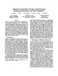
in assignment statements (equations that model the problem), 9 data taking a finite number of values, which can be represented by logical variables. These are either filters necessary to switch the computation in terms of the context (modelled domain), or tags allowing to minimize errors risks about the precision of the output values. Figure 1 shows an example of program reduction. The code section of figure 1-a is extracted from one of the applications we have studied [Nicolas&al.89]. The partial evaluation of this code section according to the simplification criteria of f'~xre 1-b yields the code section of figure 1-c. A maintenance team is used to update a specific version of the application. These people know some filters properties (IC = 0 and IREX = 1 ) as well as data about geometry ( D X L U = 0, 5 ). Furthermore IM is a tag whose value is 20. The knowledge of these values of input variables simplifies the code (as shown in figure 1c). Because of the truth of the relation I R E X = 1, two alternatives are simplified (1). The first alternative is simplified to its then-branch. In this branch, the variable DXLU is replaced by its value, which modifies the variables X(I) and DX(I) (2). The variable IM is replaced by its value too (3). The condition of the next alternative is simplified (4) since the value of IC is known. Furthermore, the relation IC = 0 simplifies the following alternative to its then-branch (5), which allows to compute the value of the variables 7.k-9,O, IREGU and IDECRI (6). Because the values of these three variables axe constant values, the three corresponding assignments are removed from the code. Then other alternatives are simplified (7).

187

(i) (3)

(2) (3) (2)

W(IREX ~E. 0) THEN DO 111 , I = 1 ,IM X(I)= XMIN + FLOAT(I-I) * DXLU [11 CONTINUE DO 1 1 2 , I = 1 ,IM DX(1) = D X L U * I

ELSE R E A D (NHC11,*, ERR=If03) X D O 121 ,I= I ,IM DX(1) = X(I+l) - X(1)

(5)

(6)

(i)

(6) (7)

(7) (7)

,=

1

IC = 0

1M - 20 DXLU

[12 C O N T I N U E

(4) (6)

WEX

,,

0, 5

Fig. 1-b. Cmmtraints on

input variables

L21 CONTINUE ENDIF IF ( IMATSO .EQ. 0 .AND. IC .OE. 0) THEN ZERO =0.

IF (IC.EQ. 0) THEN IREGU = 1 ELSE IF (IC .GE. I ~ THEN IREGU-- 0 ENDIF IF ( I ~ _ ~ .EQ.2 ) THEN READ (1~C1I,'(A)',ERR=5,END=-5)I IF ( INDEX(L,'I') .NK 0 ) THEN IDECRI = 1 ENDIF ELSE IDECRI = 2 ENDIF IV ( mECRI .EQ. 1 ) T H ~ IF (IREGU .EQ. 0) IMIN=2 IMAX =IM ELSE IMIN=IM IMAX = IM ENDIF ELSE IF ( IDECRI .EQ. 2 ) THEN IF ( IREGU .EQ. 0 ) THEN JMIN= 2 JMAX = JM ELSE JMIN-- JM JMAX = JM ENDIF ENDIF ENDIF

Fig. 1-a. Initial code

DO 111 . I = 1,20

X(1) =XMIN + O,5*FLOAT(I-I ) i 11 CONTINUE DO 112 . I = 1.20 DX(D = 0,5"1 t 12 CONTINUE IF ( IMAT$O .EQ. 0 ) THEN JMIN --JM JMAX = JM ENDIF END

Fig. 1-c. Simplified code

Fig. 1. An example of program simpfification

188

This reduction is specially important thanks to the high number of assignments and conditionals. This is the case for most subroutines implementing mathematical algorithms. For subroutines whose main purpose is editing results or calling other subroutines, the reduction is generally not so important. The links between the initial code and the simplified one are not shown in figure 1. But, if the user wishes to see how the simplified code has been obtained from the initial one, he can visualize both codes in a same window in which the simplified code is written in a different colour.

3. Two Aspects of Partial Evaluation Applied to Imperative Programs Our partial evaluator performs two main tasks: constant propagation through the code and simplification of statements. The tool can execute one of the two independently of the other. For instance, if the user is a physicist who is familiar with the equations implemented in the code, he wishes to locate in Fortran statements these equations and their variables, as they appear in the formulae of these equations. But if the user is a maintainer who does not know the application well, he would rather visualize the code as simplified as possible. In most cases however and for an optimal partial evaluation, the tool performs both tasks. 3.1. Constant Propagation Constant propagation is a well-known global flow analysis technique used by compilers. It aims at discovering values that are constant on all possible executions of a program and to propagate forward through the program these constant values as far as possible. Some algorithms now exist to perform fast and powerful constant propagation [WegmanZadeclO1]. We describe in this section our constant propagation process. It modifies most expressions by replacing some variable occurrences by their values and by nonnalising all expressions through symbolic computation. Presently, our tool propagates only equalities between variables and constants. Of course, that limits the precision of the analysis. Substitution. Before running the partial evaluator, the user specifies numerical values for some input variables of the program (thanks to his personal knowledge of the application). Constant propagation spreads this initial knowledge supplied by the user. In a first stage, the partial evaluator replaces each specified variable by its value. Then, expressions whose operands are all constant values are computed and these resulting values are propagated forward through the whole program. This technique allows to remove from the code all occurrences of variables identifiers that are not meaningful. The substituted values may be visualized differently from other values (with a different colour). Normalisation. For any numerical expression, we have to recognize if it reduces to a constant value (e.g. x+3-x reduces to 3). In the same way, for any logical expression, we have to recognize if it reduces to a conjunction of equalities or to a disjunction of inequalities, h the fast case (respectively the second case), we will be able to propagate equalities in the then- (respectively else-) branch of alternatives. To do this, we perform constant propagation. To propagate constant values as most as possible, our system

189

normalises each expression into a canonical form: a polynomial form for numerical expressions and a conjunctive normal form for the logical expressions. In a polynomial form, expressions are simplified by computing the values of the coefficients of the polynomial. Polynomial forms are written according to the decreasing powers order. When some terms of a polynomial have the same degree (e.g. z2, x2 and t.u), they are sorted according to a lexicographical order (e.g.t.u < xZ< z2). The canonical form of a relational expression is obtained from the canonical forms of its two numerical subexpressions. In normalized relational expressions, all variables and values occur on only one side of the operator. Because of these modifications of expressions, overflow, underflow or round-offerrors may happen. Therefore, the normalization of expressions may cause run-time errors. It is possible to obtain programs that will cause machine errors when compiled and executed. Conversely, some run-time errors may vanish thanks to the partial evaluation. As most partial evaluation systems [KemmererEckroann85], our tool ignores such problems. In this case only, the tool does not yield a program which behaves like the initial one. 3.2. Simplification Simplification is an option of the partial evaluator. First, the expressions are simplified by the propagation as explained above. Then, the simplification process reduces the size of the code by removing both assignments of variables which can be evaluated to constants and statements which are never used for the specified values. This simplification includes the elimination of redundant tests and in particular the simplification of alternatives to one case thanks to the evaluation of their conditions. To simplify a statement means to remove or to modify it. Its components must be simplified, but in different contexts. This section defines the simplification for each statement. A write statement is simplified by simplifying its parameters that are expressions. A read statement is simplified by removing its parameters whoso values are known input values. If all its parameters have known values, the read statement is removed (replaced by an empty statemenO. Since the removed parameters do not appear in the residual program any more, their initialization is not missing in the code that is therefore stiU executable. An assignment simplification consists in removing it, if its expression has been evaluated to a constant.

An alternative is simplified into one of its branches when its condition has been evaluated to either true or false. Otherwise, the statements of the two branches are simplified. In this case a branch may become the empty statemenL Loops that are never entered are removed. When discovered, infinite loops are left unchanged. Otherwise, if some loop invariant holds, the only statements of the loop which are simplified by the knowledge of variables values, are those statements whose all variables belong to the invariant. Thus, we do not expand loops because we want to keep the original structure of the code. Furthermore, Fortran loops are implemented using labels and goto statements. So, when a loop is removed, its label statement is kept since other statements may contain goto statements to such labels (the label is left unchanged and the statement is replaced by a skip statement).

190

A call statement simplification consists in replacing its actual parameters whose values are known by these values. The identifier of the called subroutine is left unchanged in the current program (subroutines arc not specialized) and the user has to run the partial evaluator on this subroutine code if he wants to simplify it too. The partial evaluation does not simplify other statements. Let us notice that our tool yet can neither deal with inequalities nor with literal values.

4. Inference Rules for Partial Evaluation To specify the partial evaluation, we use inference rules operating on the Fortran abstract syntax and expressed in the natural semantics formalism [Kahn87], augmented by some VDM [Jones90] operators. This section first presents rules defining on the one hand the constant propagation process and on the other hand the simplification process. Then, it details the rules for partial evaluation of statements. These new rules combine the propagation rules and the simplification rules. Let us notice that the techniques we implement are not new, but we specify and use them in a novel way. 4.1. Propagation and Simplification Rules In the following, we use sequents such as H ~- I : H ' (propagation), H ~- I > I' (simplification), and the combination of both H [- I ~ I', H ' (propagation and simplification). In these seqnents: 9 H is the environment associating values to variables whose values are known before executing I. It is modelled by a VDM-like map [Jones90], shown as a collection of pairs contained in set braces such as [variable ~ constant.... 1, where no two pairs have the same first elements. Our system initializes such maps by the list of variables and their initial values, supplied by the user. 9 I is a Fortran statement. 9 I' is the simplified statement under the hypothesis H. 9 I-I' is H which has been modified by the execution of I. The sequents H ~ - I : H ' express the propagation relation. The sequents H ~- I: > r express the simplification under hypotheses. It depends of the components of I, which are themselves simplified under other hypotheses. Thus. the definition of the simplification relation uses the definition of the propagation relation. In the sequents, we use the map operators dora. u. t , '(I and 9 The domain operator dom is the set of the first elements of the pairs in the map. 9 The union operator u yields the union of maps whose domains are disjoint (this operator is undefined if the domains overlap). 9 The map override operator t yields a map which contains all of the pairs from the second map and those pairs of the fLrst map whose first elements are not in the domain of the second operand.

191

The map restriction operator ~ is defined with a first operand which is a set and a second operand which is a map; the result is all of those pairs in the map whose ftrst elements are in the set. 9 When applied to a set and a map, the map deletion operator ~ yields those pairs in the map whose fast elements are not in the set. The example of figure 2 illustrates these definitions.

d o m ( m ) = {X,B}

m = { X ---> 5,B ---> t r u e }

mw {Y--->7} = {Y---> 7,X---> 5,B---> t r u e } m =

(x

{B}~m = {x n = {C--->false,X---> 8}

5} 5}

{B --e true,C --->false, X --->8}

HI'~ il

=

ntm

= {B ---> true,C --->false, X - e 5}

Fig. 2. Some map operators We have written some rules to explain how sequeuts are obtained fi'om other sequents. A rule is composed of a possibly empty set of sequents on the numerator, the rule premises, and of a sequent at the denominator, the conclusion of the rule. If the premises hold, then the conclusion holds. The rules we present in figure 3 express the simplification of logical or numerical expressions. They belong to the eval system, which is a subsystem of the simplification system .-.-.~. The first rule has no premise. It specifies that a variable X which belongs to the environment is simplified into a constant which is equal to its value C. To evaluate an expression E 1 0 P E2 to the value T, its two operands E1 and E2 must have been evaluated to E' 1 and E'2 respectively, and the value T is the result of the computation of E' 10P E'2 (through the comp system). If E'I and E'2 are both constants (respectively N1 and N2), the computation of T is processed by the application of the app primitives to the operator OP and to its two operands N1 and N2.

192

FT q HU{X-->C}~

id(X)

> C

comp H~

E1

>E'I

E2 ~

H~

.F

E'2

E 1 0 P E2

~ O P , E' 1, E'2: T > T

E'i r number (N) for i=1,2

comp ~ O P , E' 1, E'2: E'I OP E'2

app

(OP,NI,N2,T)

comp OP, number(N1), number(N2): T with

f

app (+, I, J, number(Z)) :- Z is I + J app (-, I, ~I, bool(true)) :- I = J app (-, I, J, bool(false)) :- not (I = J)

by using C-Prologlike evaluationpredefinlteprimitives. Fig. 3. Simplificationof expressions The rule of figure 4-a expressesthe propagationthrougha sequenceof statements. To propagate the environmentH throughthe sequenceof statementsI1;I2, H is propagated through the statementI1, whichupdates H in H1. This new environmentH1 is propagated through I2, whichupdatesH1 in 14_2.I-I2is the environmentresultingfrom the propagation through the sequence.

H ~ Ii:HI

HI~ 12:H2

H ~11;12:H2 Fig. 4- a. Propagation through a sequence of statements

193

The rule of figure 4-b expresses the simplification of such a sequence. Given an environment H, to simplify a sequence of statements I1;I2 the first statement I1 is simplified in I' 1, and the environment H is propagated through I1. In this new environment H1, the second statement 12 is then simplified.

H ~ Ii >I'I

H ~ II:HI

H ~ 11;12

HI~12

>1,2

> 1'1;1'2

Fig. 4- b. Simplification of a sequence of statements Figure 5 presents some simplification and propagation rules for alternatives. If the condition C of an alternative evaluates to true. then: 9 the environment H' resulting from the propagation of H through the alternative is obtained by propagating H through the statements of the then-branch (first rule: propagation), 9 the simplification of the alternative is the simplification of its then-branch (second rule: simplification). The last rule of f~,ure 5 is a propagation rule. It shows that information can sometimes be derived from the equality tests that control alternatives. If the condition of an alternative is expressed as an equality such as X=E, where X is a variable that does not belong to the domain of the environment H and E evaluates to a constant N, then this equality is added to the environment related to the statements of the then-branch (but this equality is not inserted as assignment in the code). There is a corresponding rule for a condition of an alternative expressed as an inequality such as X-E: this condition is transformed in an equality such as X=E which is added to the environment related to the statements of the else-branch. Such rules have been generalized to conditions of alternatives expressed as conjunctions of equalities and disjunctions of inequalities. The last rule expresses that only equalities between variables and constants can be added to the environment. Thus, if other information are expressed in the condition, they are not taken into account by the partial evaluator.

194

eval

H~

C ~ ,true

H~

II:H'

H ~ if C then I1 else 12 fi: H' eval

H~

C

>true

H~

IX

H ~" if C then I1 else 12 fi

>I'1 > I' 1

eval

H~ E

> number(N)

X ~ dom(H) Hk_){X---~N}~ II:H1 H ~ I 2 : H 2

H ~ if (X = E) then I1 else I2 fi: H l n H 2 Fig. 5. Some rules for alternatives The propagation does not depend on the simplification. But since the simplification is performed in the context of the propagation, we have chosen to represent rules grouping propagation and simplification. They are very close to the rules we have implemented in the Foresys [Foresys93] toolkit, which compile them into Prolog. Foresys has been built upon the Centaur/Fortran environment [Centaur90]. 4.2. Combined rules For every Fortran statement, we have written rules that describe the combination of the propagation and simplification systems. This combination ~ of these two systems is defined by: H I - I - - - - - - - ~ I',H'

iff

H I - I:H'

and

HI- I

>I'

From this rule, we may define inductively the ~ relation. For instance, figure 6 shows the rule for a sequence of statements. A sequence is evaluated from left to right: The partial evaluation of a sequence of two statements I1 and 12 consists in simplifying I1 in I'l then in updating (add, delete or modify) the data environment H. In this new data environment H1, I2 is simplified in 1'2 and HI is modified in H2. H ~ I1--------~ I ' I , H1

H 1 ~ I 2 --------~I'2, H2

H ~ I1; I2------~ I'l; I'2, H2 Fig. 6. Partial evaluation of a sequence of statements

In the sequel of this paper, we call such rules partial evaluation rules.

195

F i g ~ 7 specifies the rules for partial evaluation of assitrnments.The eval notation refers to the formal system of rules which simplifies the expressions, that we have previously presented. If the expression E evaluates to a numerical constant N, the ass~nment X := E can be removed in the simplified program, and the data environment H is modified: the value of X is N whether X had already a value in H or not. If E is only partially evaluable in E'. the expression E is modified in consequence in the assiL-,nmentX:= E and the variable X is removed from the environment if it was in it.

eval H ~ E

> number(N)

H ~- X := E ~

eval H ~- E H~"

> E' X : = E ~

skip, Ht{X-->N}

E' ~ number (N) X:=E',{X}'~

H

Fig. 7. Partial evaluation of assignments The following examples illustrate these two cases. In example Ex.1, as the value of the variable A is known, the assignment C := A+ 1 can be removed from the simplified program and the new value of the assigned variable C is introduced in the data environment. In example Ex.2, after the partial evaluation of the expression A+B, the value of C has become unknown. Such a case only happens when A and B do not have both constant values.

Ex.1

{A---> 1, C--> 4 } ~ C := A + 1 - - - - ~

Ex.2

{ A---> 1, C---> 2 } ~ C := A + B . - - - - ~ C : = I + B , { A---> 1 }

skip, { A ---> 1, C --->2 }

The rules for partial evaluation of alternatives are defined in figure 8. If the condition C evaluates to a logical constant, the alternative with condition C can be simplified to the corresponding simplified branch. If C is only partially evaluated in C', the partial evaluation proceeds along both branches of the alternative. It leads to two different environment H' 1 and H'2. Their intersection is the final environment.

196

eval H ~ C

> bool(false)

H I - I2------~,~ I'2, H '

H ~" i f C then I1 else I2 f i - - - - - ~ I'2, H'

eval

H~- I i ~

H ~ C >boo!(true)

.F eval H

>c'

if C then I1 else I2 fi ~

I'I,H' I' 1, H'

q-I1--- i,1,H,1 r Fi2-- I'2,w2

c'.bool(B)

i f C then I1 else I2 f i - - - - ~

i f C ' then I ' l else I'2 fi, H ' I n H ' 2

Fig. 8. Partial evaluation of alternatives As for alternatives, the rules for partial evaluation of loops, presented in figure 9, depend on the ability to evaluate the truth or falsity of the condition C from the current environment H. The first rule specifies that if the loop is not entered, it is removed from the code. There is no specific rule for the case where C evaluates to true, because we do not expand loops, not to alter the structure of the code. Figure 9 shows the rules for while-statements, but similar rules exist for repeat-statements. In the second rule, if C evaluates in C' (and the value of C' differs from false), the statements I of the loop can be simplified, given H resD:icted to a loop invariant Inv(I). lnv(I) is a pessimistic estimation of the variables that are not modified in the loop. It is calculated by the partial evaluator and consists in a list of variables whose values are known and that are neither in a left-hand side of an assignment, nor a parameter of a call ~ a read statement. The sequent that transforms I into I' belongs to the simplification system. Since we have imposed a pessimistic loop invariant, we did not write a sequent referring to the system : performing the propagation through I would not have modified the restricted environment.

eval H ~ C

-F

> boot (false)

while C do I end ~

skip, H

eval Inv(I)~ H ~

C

>C'

C'r

H ~ while C do I end ~

Inv(I)~ H ~ I L > I ' while C' do I' end, InvfI)d...4 H

Fig. 9. Partial evaluation of while-loops

197

5. Conclusion We have used partial evaluation for programs that are difficult to maintain because they are too general. Specialized programs for some values of their input variables are obtained by propagating these constant values (through a normalisation of the expressions) and by performing simplifications on the code, for instance assignments are removed and alternatives are reduced to one of their branches. This technique helps the maintainer to understand the program behaviour in a particular context. The residual program is furthermore more efficient because many statements and variables have been removed in it, and no additional statement has been inserted. Another advantage of this technique is that it can also be applied to abstractions at a higher level than the code. Let us notice that our tool may be used in two ways: by visualizing the residual program as a part of the initial program (for documentation or for debugging) or by generating this residual program as an independent (compilable) program. We are now focusing on the possibility for the user to supply general properties about input variables. These general properties are relational expressions composed of some literal values (e.g. x