The Visual Computer manuscript No. (will be inserted by the editor)
Stef Busking · Anna Vilanova · Jarke J. van Wijk
Particle-Based Non-Photorealistic Volume Visualization
Abstract Non-photorealistic techniques are usually applied to produce stylistic renderings. In visualization, these techniques are often able to simplify data, producing clearer images than traditional visualization methods. We investigate the use of particle systems for visualizing volume datasets using non-photorealistic techniques. In our VolumeFlies framework, user-selectable rules affect particles to produce a variety of illustrative styles in a unified way. The techniques presented do not require the generation of explicit intermediary surfaces. Keywords Visualization · Non-Photorealistic Rendering · Volume Rendering · Particle Systems
1 Introduction The visualization of large 3D volumetric datasets is an important challenge. Commonly, these visualizations use models based on reality. However, recently it has been shown that the use of illustrative techniques may provide more insight (e.g., [1], [3]). Non-photorealistic rendering (NPR) focuses on increasing the expressiveness of computer graphics by incorporating techniques adapted from traditional art and illustration. By removing unimportant details and visual clutter, NPR can direct the viewer’s attention towards the most important aspects of an image. Alternatively, NPR methods can be used to provide context to other types of visualization. In figure 1 we have used different illustrative techniques to show both focus (skull) and context (skin). The sparseness of the selected pen-and-ink styles provides a good alS. Busking Delft University of Technology E-mail:
[email protected] A. Vilanova Technische Universiteit Eindhoven E-mail:
[email protected] J. J. van Wijk Technische Universiteit Eindhoven E-mail:
[email protected]
Figure 1 Illustrative volume visualization of the Visible Male CT head dataset, combining several NPR techniques.
ternative to the translucency commonly used in methods like direct volume rendering. The image shown was rendered at interactive speeds, enabling easy exploration of the data. In existing research, surface-based NPR techniques are often adapted to work on surfaces extracted from the scientific volume datasets, such as iso-surfaces. These techniques require a geometrically defined surface. Another commonly used approach is Direct Volume Rendering (DVR). Here, non-photorealistic techniques such as lighting models are used to enhance features in the image (e.g., [10], [2], [3]). DVR is able to visualize ranges of data rather than just a single surface, but designing good transfer functions (which map data values to colors and opacities) is far from trivial. Point based methods, without using explicit surface representations, have become increasingly popular in computer graphics (see, for example, [15]). Particles, like points, are
2
entities encapsulating a 3D position and related information. However, particles are more general, as their visual representation can be selected freely. In this article, we therefore explore a purely particle-system based approach to volume visualization using NPR techniques. Particle systems offer simplicity and flexibility, and have been used as the basis for specific NPR techniques in the past (e.g., [7]). We investigate the appropriateness of a particle system for the visualization of volumetric data. The use of particles enables us to visualize surfaces and ranges of data with relatively low processing costs (enabling an interactive system). Particles offer a way of visualizing volume data more directly and flexibly than surface-based approaches. We introduce the VolumeFlies framework, which is based on particle systems that operate directly on the dataset. Different illustrative visualization techniques can be implemented within this framework by using different rules that affect properties of the particles such as their position and appearance. Our framework is inspired by the Smart Particle concept by Pang and Smith [20]. The Smart Particles are a combination of a particle systems and behavioral animation. It allows particles to be programmed to actively seek and visualize specific features in a dataset. This concept was also successfully applied to shape modeling [26]. We aim to show that a particle-based approach to volume visualization results in a flexible system and a unified way of describing various NPR techniques. We contribute several new approaches for particle-based illustrative visualization. In the following, we first give an overview of research related to our work. Next we present our framework and shortly discuss the pre-processing steps common to all visualizations. We then present a new hidden surface removal algorithm for particles, followed by the various nonphotorealistic techniques that have been implemented in our framework. Finally, we present and discuss results obtained with our prototype implementation of the framework, and give possible directions for future research.
2 Non-photorealistic rendering The body of NPR research is quite extensive. In this section we focus on techniques that have been applied specifically to visualizing volume datasets. Aside from DVR-based methods, a few researchers have presented alternative techniques that work directly on the volume data. A popular choice of NPR styles in this area is the family of pen-and-ink styles. Common elements in these styles are stippling, hatching and silhouettes. The sparseness of these elements is particularly suitable for avoiding clutter in images. Stippling is an often applied NPR technique for visualizing surfaces (e.g., [8], [24], [1]). However, the resulting images often lack detail due to the simplicity and sparseness of the stipples. On the other hand, these properties make the technique suitable for illustrating surfaces that provide context to a visualization. Another application of stippling is to visualize ranges of data, as shown by Lu et al. [17]. In
Stef Busking et al.
their system, the number of stipples drawn in each voxel was carefully adjusted to control density and shading, and to enhance features such as boundaries and silhouettes. Because little user interaction is required, their method is suitable for quickly previewing volume datasets. Unfortunately, the images often look noisy and lack detail, partly due to the lack of hidden-surface removal. Another commonly used pen-and-ink style for surfaces is hatching. Hatches drawn over a surface serve not only to provide shading, but can also directly convey shape information, for instance by using curvature to guide hatch directions [13]. Hatching is commonly implemented through procedural textures (e.g., [27], [22]), or by tracing lines over the surface (e.g., [12]). Methods have also been presented to create hatching images directly from volumetric datasets [19], [9]. The algorithms used, however, are usually computationally expensive. Most of these techniques also include silhouette extraction in order to highlight the boundaries of objects. Silhouette extraction is one of the most useful techniques in nonphotorealistic rendering. By tracing the external and possibly internal silhouettes of objects, these objects are emphasized in the visualization without cluttering their interior. A number of techniques exist for drawing silhouettes, e.g., using DVR transfer functions [14], image-based filtering [27], [29], or marching lines [4]. Yuan and Chen [29] illustrated surfaces in volume data using a combination of several techniques, including DVR, iso-surface extraction and image-based techniques. The NPR techniques work well for highlighting specific surface features in the volumes. However, using image-based methods (e.g., for extracting silhouettes) has the disadvantage that such methods only work on the front-most parts of visible surfaces in the data, and a change in viewing position requires the techniques to be re-applied. From the work described above, it seems that combinations of different styles are most useful for visualizing features in a dataset. Therefore, we investigate whether a particle-based framework is general enough to support a large variety of styles.
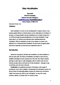
3 The VolumeFlies framework The VolumeFlies framework, shown in figure 2, consists of a four-stage pipeline. In the feature location stage, the features that we want to visualize are located and particles are created at locations on those features. Once the features (e.g., some type of surfaces) have been located, the particle manipulation stage prepares the particles for visualization. For instance, the particles will often have to be redistributed in order to cover the entire feature. Afterwards, the filtering stage can be applied. The particles in the system can be filtered based on criteria such as removing particles located at hidden surfaces. Finally, in the rendering stage, geometry is created for each of the remaining particles in order to achieve a desired visual style. Multiple sets of particles with
Particle-Based Non-Photorealistic Volume Visualization
3
VolumeFlies Feature location
Volume data Particles
Particle manipulation
Filtering
Image
(a) before
(b) after
Figure 3 Particles before and after redistribution Rendering
Figure 2 The VolumeFlies framework
different properties can be used in a visualization, in order to visualize multiple features. The geometry resulting from each of these instances is then sent to the rendering pipeline to be projected onto the final image. Each of these stages gives rise to a class of pluggable modules implementing a set of rules to be applied to the particles. These can be used as building blocks, to adapt the framework to a specific visualization scenario. The first two stages are typically performed in a pre-processing step. During rendering, the modules selected for the third and fourth stages are invoked as necessary for each change in the viewing direction and / or other visualization parameters. In the next sections we present several variations for the modules of the different stages. An important property of the modules discussed in this article is that the rules applied to each particle use only information local to that particle’s position. This improves scalability of the system to larger datasets; performance is only determined by the number of particles in the system, which is controlled by the user rather than by the data. This is a desirable property, as the density of particles influences both the scale of details visible in the data, as well as creating certain visual effects. The only exception to this is that some modules require information about neighboring particles. In this case we use a spatial binning algorithm for fast access to these neighbors.
opposite sides of the iso-surface value, the surface must intersect the line between the two points. Linear interpolation is used to approximate the location of this intersection, and a particle is created at that location. This method usually results in an uneven distribution of particles over the feature surfaces, causing visual artifacts such as the rings in figure 3(a). To solve this, we use a particle distribution method originally developed by Witkin and Heckbert [28], and later improved by Meyer et al. [18] to redistribute the particles over the surface. This is accomplished by having particles locally repel each other, but constraining them to the surface. We adapt Meyer’s improved algorithm from the context of rendering implicit surfaces to that of volume datasets and iso-surfaces by using (linear) interpolation. It is worth pointing out that the even distribution of particles on the surface (as shown in figure 3(b)) does not result in a regular distribution in image space, as regions more perpendicular to the screen will appear denser. In certain situations however, creating such a distribution is not as important, and the goal is merely to remove the patterns created by the feature location algorithm step. In some of these situations simply moving the particles in random directions over the surface for a number of steps will often produce acceptable results, and the more computationally intensive distribution method may be avoided. These steps may be computationally expensive, and furthermore, the values of the interesting iso-surfaces may not be known in advance. Therefore we implemented a second method for quickly previewing datasets and locating features of interest. Here, in the first stage an initial set of particles
4 Feature location and particle redistribution The first step is to place a set of particles at some initial position on the features we want to visualize. In medical volume data, the most commonly visualized features are isosurfaces. Therefore we chose iso-surfaces as the first implementation for the feature location module. We sample the dataset at a user-defined grid, using interpolation between data points where necessary. In this way we can ensure regular sampling in all directions even if the voxels in the original dataset are not isotropic. We identify the location of the iso-surface by comparing the value at each grid point to its direct neighbors. If these values lie on
Figure 4 Exploring a CT head dataset using non-surface particles (with silhouette extraction) and a user-configurable density transfer function.
4
Stef Busking et al.
(a) Showing all particles
(b) Hidden surfaces removed
Figure 5 Removing particles located on normally hidden surfaces can help to produce a clearer image.
is created at random locations throughout the volume where the magnitude of the gradient exceeds a certain threshold. An additional filtering stage module is added to apply a density transfer function. This is similar to an opacity transfer function in DVR; particles are hidden or shown based on the value of this function when applied to the data value at the particle’s position, using the density controlling algorithm described in section 6.1. This way, selected ranges within the data can be visualized quickly. While the amount of detail shown in the resulting images is low (see figure 4), the interactivity provided by manipulating the density function allows a user to easily identify features of interest in a volume.
5 Hidden-surface removal The most obvious issue when dealing with surfaces illustrated by separate particles rather than a complete surface (e.g., a polygonal representation) is that there is no occlusion between the rendered surfaces. While in some cases this may provide additional insight into the structure of the feature, it could clutter the image in other cases (see figure 5). Particles on hidden surfaces should be detected and (optionally) removed in the filtering stage of the framework. Most surface-based methods solve this problem by first rendering the polygonal representation of the surface to a depth buffer, and subsequently testing each of the particles against this buffer to determine their visibility. The polygonal surface can also simply be rendered using the background color in order to erase any particles that should not be visible. An alternative technique, used in [21], first renders the polygonal surface in uniquely colored patches. Particles are only deemed to be visible if the color of their corresponding patch is found in the resulting image. While this scanning approach may be slower than the depth-buffer based approach, it has the advantage that the set of visible particles can be determined before they are rendered. This makes it easier to combine different visualizations (sets of particles) in the same image. Also, using this method avoids depthvalue precision issues, a common problem with the first approach.
(a) Splats on surface (side view)
(b) Resulting / missing particles
Figure 6 Overlap between neighboring splats can cause visible particles to disappear (shown in red).
We show that hidden particles can also be removed without an explicit construction of polygonal representations of the surfaces. A common technique for rendering surfaces from separate points (point-based rendering, see for example [23], [6]) is splatting. Discs are aligned with the surface and drawn at the positions of the points. If enough discs are used and the discs are large enough, this results in an approximation of the surface. If the surface is strongly convex, disks can undesirably mask neighboring particles as shown in figure 6. This may cause gaps to appear in the surface. Using a scanning approach, this does not matter as long as some part of the discs for these particles is visible. However, in some cases the complete disc is occluded erroneously. This is especially an issue if the splatting image is generated at a lower resolution than the final image, in order to increase performance. We use the scanning approach for detecting visible particles. Our goal is therefore to find an algorithm that minimizes overlap problems between neighbors and still works well at reduced resolutions. Our solution is to use cones oriented towards the viewer rather than circular disks. The cones are scaled at their base to match the projection of the original discs (see appendix A.1 for details). The 3D nature of their shapes leads to more evenly sized projections for each particle (figure 7). In fact, when the surface is parallel to the screen, the resulting image is a Voronoi diagram of the set of particles [11]. We call this new method cone-splatting.
Figure 7 Cone splatting compared to normal splats
Particle-Based Non-Photorealistic Volume Visualization
(a) Scale-based shading
(b) Density-based shading
5
(a) Single direction
(b) Principal curvature
Figure 8 Stippling methods
Figure 9 Hatching methods
In figure 6(b), the red particles were marked visible by our cone splatting algorithm, but not by using normal splats. Two parameters control the size of the cones. The radius (of the discs used to scale the cones) needs to be large enough to create a closed surface in the projection. However, it should not be larger than the distance between neighboring particles, as this could cause cones to stick out from the surface. Increasing the axis length of the cones increases the robustness to high-curvature areas such as shown in figure 6. However, if the cones are too long (compared to the distance between subsequent faces along the viewing direction), particles behind the front-most surface may become visible undesirably.
of the lighting equation as a scaling factor for the size of a particle (see appendix A.2 for details). Another method of shading in stipple drawings is to increase or decrease the density of stipples in certain areas in order to achieve darker or lighter tones respectively (figure 8(b)). We assume that the full set of particles is sufficient to generate a black tone. As all particles are of equal size and evenly distributed, the fraction of particles shown is linearly related to the tone. We therefore first assign to each particle pi a value vi from a uniformly random distribution ranging between 0 and 1. During rendering, a particle is drawn only if the value of its lighting equation is less than this value. A disadvantage of this method is that it may require a very dense set of particles in order to create a detailed image. Very large numbers of particles affect performance as well as accuracy. On the other hand, the method is suitable for illustrating surfaces that provide context to a visualization (for example, the skin in figure 13). Transparent surfaces can also be visualized using this method. By placing the light source at the same position as the camera, silhouettes are enhanced while particles are removed from interior areas, reducing clutter. The results of both stippling methods can be improved further by observing that in traditional illustration very bright areas often contain no points at all. We can achieve this effect by removing points altogether, if their brightness is above a certain threshold.
6 Rendering Traditional medical illustrations, e.g., those used in anatomy books, commonly use pen-and-ink styles. Common elements in these styles include stippling, hatching and silhouettes. We adapt existing techniques and introduce new algorithms to emulate these styles using our particle-based framework. 6.1 Stippling The simplest way to visualize a set of particles is by using point primitives. The set of particles provides us with a set of positions in 3D space, which can be projected onto the image plane using any desired projection method in the rendering stage of the framework. Additionally, the surface normal – derived from the local gradient – can be used for applying shading, to better illustrate the shape of the surface. There are several options. In traditional illustration, two techniques are typically used to create shading effects in stipple drawings. One is to vary the scale of the points, using larger points to create darker areas (see figure 8(a)). We have implemented this as a rendering module in our framework, by using the value
6.2 Hatching Hatching is a technique that uses solely lines and curves to convey shape. Shading is often accomplished by varying line width and/or spacing. The direction of the strokes is used to illustrate the shape or material properties of the 3D surface that is being represented. In traditional illustration, both normal hatching (closely spaced parallel lines) and crosshatching (two or more sets of lines that may intersect each other) are used.
6
In our framework, creating hatched images consists of two steps. First, hatch lines are generated from the set of particles. This is done in the particle manipulation stage of the framework, where the hatch line is stored in the particle. Secondly, during rendering, a shading algorithm decides which of these lines should be drawn in order to create the appearance of a shaded surface. For the purposes of shading, we use the density-based method presented in section 6.1. We use the positions of the particles as seed points for hatch lines traced through the volume. A direction is selected in the local surface tangent plane, after which the position is updated by moving along that direction for some userselectable distance and repeating the process until a desired number of hatch-segments has been created. This is repeated in the opposite direction, again starting from the particle’s position. In order to be able to perform hidden surface removal on these hatches, each segment of the hatch line is linked to the nearest particle in the volume; a segment is drawn only if its linked particle is marked visible.
6.2.1 Direction of the hatches A simple method for selecting directions is to define a single 3D vector for all hatches representing the preferred direction. At each step while tracing a hatch, this direction is projected onto the local surface tangent plane in order to obtain a hatch direction. Due to the uniformity of the hatches, the resulting images look similar to images created using wood engraving (see figure 9(a)). A disadvantage is that in areas where the preferred direction is perpendicular to the surface the hatch field looks messy, as the hatch direction is not well defined. An alternative, as suggested by Interrante [13], is to use the directions of principal curvatures. We use the curvature estimation method presented by Kindlmann et al. [14] to compute curvature, but perform eigenanalysis on the resulting geometry tensor to obtain the directions of principal curvature as well as the values. While the directions of principal curvature work well for hatching on smooth surfaces, the iso-surfaces in realworld datasets (such as medical volume data) are not always smooth and often noisy. In order to obtain reliable derivatives, and to ignore unimportant details on the surface, we blur the dataset using a Gaussian kernel. This allows us to calculate curvature properties at a proper scale; the choice of the size of the Gaussian kernel depends on the scale of the details we want to visualize. To further improve our results, a smoothing algorithm is subsequently applied to the direction field. Figure 9(b) was generated using this method. Hertzmann and Zorin [12] illustrated smooth surfaces using hatching patterns. They used a complex energy minimization algorithm to produce smoothed principal curvature directions. Our smoothing algorithm, which is described in detail in the next section, is less complex but produces similar results.
Stef Busking et al.
(a) Initial directions
(b) After smoothing
Figure 10 Computed curvature directions on the chin of the CT head dataset
6.2.2 Smoothing the direction field One problem with principal curvature directions is that they are not well defined in areas where the surface is flat or (nearly) spherical. Moreover, Hertzmann and Zorin [12] have noted (based on hatching patterns in traditional illustration) that hatching using principal curvature directions is most effective in areas that are parabolic. That is, areas where one of the principal curvatures (κ1 and κ2 ) is large while the other is near zero. If one of the curvatures is exactly zero the surface is locally cylindrical. Based on these observations, we have designed a new smoothing algorithm which generates direction fields suitable for hatching. Like Hertzmann and Zorin, we use a crossfield consisting of unordered pairs of directions, because there are certain cross-hatching patterns that can not be decomposed into two separate single-direction fields. The field is stored as a pair of direction vectors in each particle. While tracing a hatch, the field from particles near the current position is averaged to obtain an approximate pair of directions for that point. We then select the direction most like the current hatch direction as the direction in which to continue the hatch line. The field is initialized with principal curvature directions. As can be seen in figure 10(a), there are several areas where this field contains irregularities due to noise or ill-defined principal curvature. We define a measure of field reliability, ρ , which essentially states how suitable for hatching the principal directions are at a given point. We base this measure on the shape index s, defined by Koenderink and Van Doorn [16], 2 κ 2 + κ1 s = arctan (κ1 ≥ κ2 ) . π κ2 − κ1 The shape index is a number between −1 and 1 indicating the shape of the surface. We transform s into our reliability measure by taking ρ = 1 − |2 (|s| − 1/2)|. The value of ρ ranges from 0 (spherical or saddle-shaped) to 1 (cylindrical). This way, when ρ = 1, the principal curvature directions are most suitable for hatching, while ρ = 0 means the directions are unreliable. The shape index does not indicate whether a surface is flat, that is, if both κ1 and κ2 are (nearly) 0. It is, however, important to detect flat areas as the directions of principal curvature are not well defined in those areas, therefore we set ρ to 0 in these cases.
Particle-Based Non-Photorealistic Volume Visualization
(a) Bones of the hand
(b) Blood vessel
7
(a) Silhouettes based on n · e
(b) Constant-width silhouettes
Figure 11 Iso-depth “silhouettes”
Figure 12 Controlling the width of the silhouette lines
We iteratively replace the directions in each particle with the average taken over that particle’s neighborhood, using the values of ρ in each particle as weights. This leads to blurring in areas of low reliability, while reliable directions are preserved. Differences in the orientation of the surface at neighboring particles may cause the averaged directions to be outside of the surface tangent plane. To prevent this, directions are rotated according to the minimal rotation between the surface normals at the particles before they are averaged. As can be seen in figure 10(b), the resulting field is more coherent than figure 10(a) in areas where the principal directions would not be well defined.
curvature direction vectors k1 and k2 combined with the local surface normal n, and using Rodrigues’ formula [25], we derive an approximation for the silhouette line in this frame (see appendix A.3). From this we obtain the direction,
6.3 Silhouette extraction In order to include silhouettes in our generic framework, we would like to use the existing set of particles. Extracting silhouettes consists of two steps. First, a subset of particles near the silhouette is selected. These can be found by placing a threshold on the dot product of surface normal n and viewing direction e. Next, we trace silhouettes in a way similar to hatching. Unlike hatching, tracing of silhouettes can not be performed in a pre-processing step, because silhouettes are dependent on the viewing direction. In order to follow the silhouette, the direction of silhouette lines should keep the surface normal perpendicular to the viewing direction. One option is to draw iso-depth lines instead of following the true silhouette. We obtain these by following the direction of n × e. This method results in a decent approximation to silhouettes for objects for which these silhouettes lie in or close to planes perpendicular to the viewing direction (figure 11(a)). In areas where this is not the case, the result is often a sketch-like effect (see the lower bones in figure 11(a)). The method fails, however, on small cylindrical structures, such as the blood vessel in figure 11(b). The iso-depth lines can also work as an effective hatching pattern. In order to obtain more accurate silhouettes (see figure 13), we note that the local surface curvature describes the local behaviour of the normal. It can therefore be used to determine the silhouette direction. By considering a local coordinate frame at point p consisting of the principal
d = −κ2 (k2 · e) k1 + κ1 (k1 · e) k2 . Blurring is applied to improve the robustness to noise of the curvature calculation. We need to determine which particles to draw silhouettes from. Using a threshold on n · e results in wide silhouette lines in areas of low curvature, while silhouettes in areas of high curvature are smaller or may be missed altogether if no particles are in the silhouette area (figure 12(a)). Kindlmann et al. [14] observed a similar problem when drawing silhouettes using transfer functions in direct volume rendering. They proposed using a 2D transfer function dependent on not only the n · e value, but also on the local surface curvature. Their method requires the surface curvature in the viewing direction, which they derive from the geometry tensor matrix for each point whenever the viewpoint changes. We can avoid additional expensive computations by reusing our earlier approximation of the silhouette line. The distance of a particle to the silhouette can be derived from the distance of this line to the origin in the (k1 , k2 )-plane,
τ=q
n·e (κ1 (k1 · e))2 + (κ2 (k2 · e))2
.
Assuming orthogonal projection, the distance of the particle to the silhouette in the image plane is T = τ (n · e). We can therefore place a threshold on the value of T in order to obtain silhouettes of approximately constant width (see figure 12(b)). The only disadvantage is that principal curvature information has to be computed for all particles. However, as this information is independent of the viewpoint this can be performed in a pre-processing step.
7 Results The algorithms described in this article have been implemented in C++ using the OpenGL 3D graphics API [5]. The
8
Stef Busking et al.
(a)
(b)
(c)
(d)
Figure 13 Illustrative volume visualizations of a CT hand dataset, combining several NPR techniques.
resulting system allows a user to easily configure a number of sets of particles within a volume dataset, each of which can have its own visualization technique and parameters. Different techniques can be combined to visualize multiple features in a volume dataset. Figure 13 shows a CT dataset of a hand visualized using our framework. The focus of the image, the bones of the hand, are visualized using a traditional iso-surface rendering. This is rendered by splatting with a dense set of realistically shaded particles. The surface is emphasized in the image using silhouettes. This is combined with principalcurvature directed hatching in figures 13(a) and 13(c) in order to better illustrate the shape of this surface. Alternatively, stippling and silhouettes can be used to show the interior structure of the surface (figure 13(b)). Context is provided by a visualization of the skin using its silhouette, and also stippling in figures 13(a) and 13(c). Figures 13(a) and 13(d) also show the arteries in the hand (using accurate silhouettes based on curvature). Our framework is flexible enough to produce visualizations in many styles and variations, similar to results of surface-based techniques. Our current implementation is limited to visualizing iso-surfaces. However, the methods presented can be extended to other types of surfaces if the required derivative properties (surface normal and in some cases curvature) are available. The Visualization of ranges of data (rather than iso-surfaces) leaves room for improvement. Currently, these techniques seem most suitable for quickly previewing datasets. However, due to the limited amount of particles used, the resulting images offer less detail than the volumetric visualizations as used by Lu et al. [17]. DVR images often look fuzzy; transparent structures in these images may clutter the image, especially when one is mainly interested in specific surfaces within the volume. In these cases, the sparseness of our NPR techniques may offer a better alternative. Because only simple geometric primitives were used to render our results (points and lines), these two types of visualizations may also be easily combined, for instance in a focus / context type of visualization. For exam-
ple, figures 13(a), 13(c) and 13(d) show NPR combined with a surface shaded using more classical techniques. The system runs at interactive speeds (with the exception of the pre-processing steps), allowing a user to immediately observe the result of changing most of the visualization parameters. Table 1 gives an overview of the performance of the (unoptimized) prototype implementation, for some of the images presented in this article. All datasets used were in the range of 2563 voxels. Stages 1 (feature location) and 2 (particle manipulation) are pre-processing steps (executed once per dataset) while stages 3 (filtering) and 4 (rendering) are executed during interactive rendering when certain parameters are changed.
8 Conclusions and future work We have discussed a framework for particle-based nonphotorealistic volume visualization. Our main contributions are: – The VolumeFlies framework, a flexible and scalable framework for non-photorealistic rendering of volume data, based on particle systems and operating directly on the voxel data. We have demonstrated that the framework Table 1 Performance of the framework on a modern computer (AMD Athlon 2 GHz) Image Figure 1 Figure 8(a) Figure 8(b) Figure 9(a) Figure 9(b) Figure 11(a) Figure 12(a) Figure 12(b) Figure 13(a) Figure 13(b) Figure 13(c) Figure 13(d)
sets
particles
stage 1&2
stage 3&4
4 1 1 1 1 1 1 1 6 3 5 4
221108 26714 1294185 58367 58367 27070 29481 29481 449529 367921 404831 410487
120 s 15 s 360 s 35 s 60 s 15 s 20 s 20 s 130 s 90 s 120 s 100 s
2 fps 30 fps 1 fps 19 fps 17 fps 19 fps 4 fps 2 fps 2 fps 5 fps 6 fps 2 fps
Particle-Based Non-Photorealistic Volume Visualization
supports various styles in a unified way, including stippling, hatching and silhouette extraction. Other styles, such as the painterly rendering styles in [7], could also be easily implemented within the same concepts. – A new hidden surface detection algorithm for surfaces rendered using particles. This method does not require the construction of an explicit geometric representation of the surface and can be applied at interactive speeds. – New techniques for NPR and visualization, including a simple density-based shading algorithm, silhouette approximation methods and a direction field smoothing algorithm for hatching based on principal curvature directions, which uses the shape index to indicate the local suitability for hatching. Non-photorealistic methods for data visualization, such as the ones presented in this article, may be used to simplify visualizations in cases where “realistic” methods would clutter the image. They are by no means a replacement for methods such as DVR. Rather, they should be considered a useful addition, as each has its own advantages and disadvantages. We expect that non-photorealistic methods are particularly suitable to provide context for more realistic visualizations, as their inherent simplicity will serve not to distract the viewer from the focus of such an image. We also conclude that the use of particles presents a useful alternative to traditional surface-based methods. The flexibility presented by particles combined with the advantages of working directly on the data may present new possibilities for data visualization, and allows easy implementation of many NPR techniques. However, there are still topics for further research. For instance, it may be useful to adapt the density of particles to certain situations. Examples are modifying density when zooming in order to ensure a constant tone, to adapt it according to local surface properties such as curvature, or using user-defined focus regions to control density and / or other visualization parameters. Also, as shown in our experiments with alternative feature location rules, particles do not necessarily have to be on the same surface. Further research is required in order to adapt our techniques for optimally visualizing ranges of values, as is possible with DVR. Finally, the current implementation of the framework does not take advantage of programmable graphics hardware. We are working on an implementation of the framework which uses graphics hardware in order to allow for interaction during the preprocessing stages and improve the overall performance. References 1. Baer, A., Tietjen, C., Bade, R., Preim, B.: Hardware-accelerated stippling of surfaces derived from medical volume data. In: EuroVis, Proceedings, pp. 235–242 (2007) 2. Bruckner, S., Gr¨oller, M.E.: Volumeshop: An interactive system for direct volume illustration. In: IEEE Visualization, Proceedings, pp. 671–678 (2005) 3. Bruckner, S., Gr¨oller, M.E.: Style transfer functions for illustrative volume rendering. Computer Graphics Forum 26(3), 715–724 (2007)
9
4. Burns, M., Klawe, J., Rusinkiewicz, S., Finkelstein, A., DeCarlo, D.: Line drawings from volume data. In: SIGGRAPH, Proceedings, pp. 512–518 (2005) 5. Busking, S.: Volumeflies - a smart-particle-inspired framework for illustrative volume rendering. Master’s thesis, Technische Universiteit Eindhoven (2006) 6. Co, C.S., Hamann, B., Joy, K.I.: Iso-splatting: A point-based alternative to isosurface visualization. In: Pacific Graphics, Proceedings, pp. 325–334 (2003) 7. Cornish, D., Rowan, A., Luebke, D.: View-dependent particles for interactive non-photorealistic rendering. In: Graphics Interface, Proceedings, pp. 151–158 (2001) 8. Deussen, O., Hiller, S., van Overveld, C., Strothotte, T.: Floating points: A method for computing stipple drawings. Computer Graphics Forum 19(3), 40–51 (2000) 9. Dong, F., Clapworthy, G., Lin, H., Krokos, M.: Nonphotorealistic rendering of medical volume data. IEEE Computer Graphics and Applications 23(4), 44–52 (2003) 10. Ebert, D., Rheingans, P.: Volume illustration: Non-photorealistic rendering of volume models. In: IEEE Visualization, Proceedings, pp. 195–202 (2000) 11. Haeberli, P.: Paint by numbers: abstract image representations. In: SIGGRAPH, Proceedings, pp. 207–214 (1990) 12. Hertzmann, A., Zorin, D.: Illustrating smooth surfaces. In: SIGGRAPH, Proceedings, pp. 517–526 (2000) 13. Interrante, V., Fuchs, H., Pizer, S.: Conveying the 3d shape of smoothly curving transparent surfaces via texture. In: IEEE Transactions on Visualization and Computer Graphics, pp. 98–117 (1997) 14. Kindlmann, G., Whitaker, R., Tasdizen, T., Moller, T.: Curvaturebased transfer functions for direct volume-rendering: methods and applications. In: IEEE Visualization, Proceedings, pp. 513–520 (2003) 15. Kobbelt, L., Botsch, M.: A survey of point-based techniques in computer graphics. Computer & Graphics 28(6), 801–814 (2004) 16. Koenderink, J., van Doorn, A.: Surface shape and curvature scales. Image and Vision Computing 10(8), 557–565 (1992) 17. Lu, A., Ebert, D., Hansen, C., Hartner, M., Morris, C., Rheingans, P., Taylor, J.: Illustrative interactive stipple rendering. IEEE Transactions on Visualization and Computer Graphics 9(2), 127–138 (2003) 18. Meyer, M., Georgel, P., Whitaker, R.: Robust particle systems for curvature dependent sampling of implicit surfaces. In: Shape Modeling and Applications, Proceedings, pp. 124–133 (2005) 19. Nagy, Z., Schneider, J., Westermann, R.: Interactive volume illustration. In: Vision, Modeling and Visualization Workhop, Proceedings, pp. 497–504 (2002) 20. Pang, A., Smith, K.: Spray rendering: Visualization using smart particles. In: IEEE Visualization, Proceedings, pp. 283–290 (1993) 21. Pastor, O., Strotthote, T.: Graph-based point relaxation for 3d stippling. In: The Fifth Mexican International Conference in Computer Science, ENC, Proceedings, pp. 141–150 (2004) 22. Praun, E., Hoppe, H., Webb, M., Finkelstein, A.: Real-time hatching. In: SIGGRAPH 2001, Computer Graphics Proceedings, pp. 579–584 (2001) 23. Rusinkiewicz, S., Levoy, M.: Qsplat: A multiresolution point rendering system for large meshes. In: SIGGRAPH, Proceedings, pp. 343–352 (2000) 24. Secord, A.: Weighted Voronoi stippling. In: The second international symposium on Non-photorealistic animation and rendering, Proceedings, pp. 37–43 (2002) 25. Struik, D.: Lectures on Classical Differential Geometry. Courier Dover Publications (1988) 26. Su, W.Y., Hart, J.C.: A programmable particle system framework for shape modeling. In: International Conference on Shape Modeling and Applications, Proceedings, pp. 114–123 (2005) 27. Treavett, S.M.F., Chen, M.: Pen-and-ink rendering in volume visualization. In: IEEE Visualization, Proceedings, pp. 203–210 (2000)
10
Stef Busking et al.
28. Witkin, A.P., Heckbert, P.S.: Using particles to sample and control implicit surfaces. In: SIGGRAPH, Proceedings, pp. 269–277 (1994) 29. Yuan, X., Chen, B.: Illustrating surfaces in volume. In: VisSym, Proceedings, pp. 9–16 (2004)
S. Busking Stef Busking received both BSc (2005) and MSc degrees (2006) in computer science from the Technische Universiteit Eindhoven. He is currently a PhD candidate at Delft University of Technology. His research interests include computer graphics and visualization, medical or otherwise. He currently performs research into comparative visualization for medical datasets.
A Derivations A.1 Splat-cone scaling The cones used for hidden surface removal are scaled to match the projection of the original splat discs. To simplify the calculations, we assume a local orthogonal projection along the viewing direction ei . In this projection, a disc with radius r, aligned perpendicular to surface normal ni will result in an ellipsoid projection. This ellipsoid will have axis lengths r and ri0 , where ri0 = r (ni · ei ) . The orientation of the axis can be found by observing that the disc will retain its radius in the direction perpendicular to both the viewing direction and the surface normal: ri = r (ni × ei ) . The axis with length r0 is obviously perpendicular to this, so r0 i = ri0
ei × ri . |ei × ri |
A.2 Scale-based stippling
A. Vilanova Anna Vilanova is an assistant professor at the Biomedical Image Analysis group at Technische Universiteit Eindhoven. She received her PhD degree in 2001 from the Vienna University of Technology and a MSc in Computer Science from the Universitat Polit`ecnica de Catalunya. Her current research interests are in medical visualization and image analysis.
Assuming the particles are evenly distributed, they will form an approximately hexagonal pattern over the surface (recall figure 3(b)). We further assume that particles in the immediate neighbourhood of a particle pi experience similar lighting conditions as pi , and ignore overlap between particles. Consider a triangle in the hexagonal grid, consisting of particles pi , p j and pk . Our assumptions allow us to simplify the size of these particles to a single Si . This way, the fraction of white in the triangle (i.e., the intensity Li at those points) can be expressed as 1 π S2 Li = 1 − 1 2√ i , 2 4 3σ
where σ is the (average) distance between neighbouring particles. This can be solved for Si , resulting in s√ 3 Si = σ (1 − Li ). 2π
A.3 Curvature-based silhouette approximation
J.J. van Wijk Jarke J. van Wijk is full professor in Visualization at the Technische Universiteit Eindhoven. He holds a PhD in computer science (1986) and a MSc in Industrial Design Engineering (1982) from the Delft University of Technology. He is a member of IEEE, ACM SIGGRAPH and Eurographics, and has served as paper co-chair for IEEE Visualization and IEEE InfoVis.
Suppose the local principal curvatures at point p are given by κ1 and κ2 , with directions k1 and k2 respectively. These vectors, combined with the surface normal n form a local coordinate frame in p. Using Rodrigues’ formula, we can linearly approximate the behaviour of the normal in this frame: n0 (u, v) = (−κ1 u, −κ2 v) , where u and v correspond to the k1 and k2 directions respectively. The to-eye vector e can be described in this frame as e0 = (k1 · e, k2 · e, n · e) . This allows us to define the silhouette as the line e0 · n0 (u, v) = −κ1 (k1 · e) u − κ2 (k2 · e) v + n · e = 0, from which we derive a parallel direction vector in world-space: d = −κ2 (k2 · e) k1 + κ1 (k1 · e) k2 .