PARTICLE IMAGE VELOCIMETRY ERRORS DUE TO REFRACTIVE INDEX FLUCTUATIONS P. Ryan Jackson1, Rodrigo A. Musalem1 Chris R. Rehmann1, David F. Hill2 1
Ven Te Chow Hydrosystems Laboratory, Department of Civil and Environmental Engineering, University of Illinois at Urbana-Champaign, 205 N. Mathews Ave. Urbana, Il 61801; PH (217) 333-6183; FAX (217) 333-0687; email:
[email protected] 2
Department of Civil and Environmental Engineering, The Pennsylvania State University, 212 Sackett Building University Park, PA 16802; PH (814) 863-7305; FAX (814) 863-7304; email:
[email protected] ABSTRACT
Non-intrusive velocity measurements in turbulent, stratified flows are hampered by index of refraction fluctuations. These fluctuations can reduce the data rate and quality in laser Doppler velocimetry by displacing the beams. In an experiment with particle image velocimetry (PIV), the displacement of light reflected from particles can produce spurious particle positions and velocities. Although matching the indices of refraction of the stratifying agents can eliminate these problems, the costs associated with stratifying a large facility can be high. Thus, we seek to quantify the errors incurred in PIV measurements as a function of the intensity of the turbulence. We present results of a laboratory experiment in which images of a stationary target mimicking typical PIV images are acquired under different conditions. Because the target is fixed, any displacement registered by the PIV system is an error. The experimental facility consists of a salt-stratified tank stirred with arrays of vertical rods oscillating horizontally. Direct force measurements allow the work done by the rods on the water, and thus the average dissipation εa, to be estimated. Concurrent density measurements during the stirring are used to compute the length and time scales of the largest eddies. PIV errors are then expressed as a function of the turbulence intensity and the path length LP. The former quantity is measured by εa/νN2, where N is the buoyancy frequency.
INTRODUCTION
Particle Image Velocimetry (PIV) is a nonintrusive measurement technique employed to measure the velocity field in a fluid flow seeded with tracer particles. The idea behind PIV is simple: Modern PIV uses sequential images separated by small times of a seeded flow illuminated by a laser sheet and gathered by a high resolution CCD camera to provide a velocity field for a given flow. The images are processed using an algorithm that uses either auto- or cross-correlation to determine the displacement of particles from one image to the next. From the displacement and the time separation, the velocity field may be computed and displayed as a vector field. This technique hinges on accurate imaging of the tracer particles in the flow; any error in the images is transferred to errors in the velocity measurements. In turbulent, stratified flows, one source of error is fluctuations in the index of refraction, which occur because eddies create horizontal density variations. At the interface between the heavy and light fluid, light will refract a distance proportional to the density difference and cause an apparent shift in the particle location. The PIV algorithm will then return erroneous velocities. We evaluate errors in PIV due to refractive index fluctuations in turbulent, stratified flows. Refractive index fluctuations also affect other velocimetry techniques. In laser Doppler velocimetry, a technique in which the Doppler shift of light from two crossing laser beams in a fluid flow is used to compute the velocity at the crossing point, the bending of the laser beams due to the variable index of refraction causes the beams to cross only intermittently as they “wander” in the measurement region. McDougall (1979) found that the fluctuations in index of refraction caused the laser beams to migrate up to 5 mm over 2 cm of path length, resulting in loss of data and “pseudoturbulence” in the high frequency spectrum. To eliminate this problem, McDougall developed a method that matches the index of refraction of the solutions without losing the density difference necessary to drive the stratified flow. This technique has since been used by many workers (e.g. Hannoun et al. 1988, Alahyari and Longmire 1994). This method is not without limitations, however. McDougall cites the limitations are due to i) the accuracy with which one can measure the indices of refraction of the two solutions, ii) the inherent nonlinearity of the index with concentration, iii) differing molecular diffusivities of the two solutes, and iv) the high cost to stratify a large tank using this technique. Differences in the molecular diffusivities of the two solutes can lead to double diffusion, which can change the index of refraction and introduce unwanted physical phenomena (McDougall 1979). The difficulty in finding solutions that are both physically appropriate and cost efficient was pointed out by Alahyari & Longmire (1994) and Hannoun et al. (1988). They found the technique beneficial, but only after exhaustive searches for stratifying solutions. For PIV in turbulent, stratified flows several approaches have been used to deal with effects of refractive index fluctuations. Using photographic PIV, Alahyari & Longmire (1994) found that without index matching the fluctuations created blurred images in which the individual particle images could not be distinguished. Fincham et al. (1996) marked an isopycnal with neutrally buoyant particles and claimed that no
2
index matching was required. Nimmo Smith et al. (2002) limited their measurements to regions that are fully mixed as in measurements of the coastal ocean using underwater PIV. More recent work by Fernandes (2001) on thermal convection shows that errors exist for flows with a total temperature difference of 12°C or more; for smaller temperature differences, the errors were deemed negligible for his application. However, since these results apply only to these convection experiments, we quantify the magnitude of these errors in terms of the strength of the stratification and the intensity of the turbulence so that future workers can confidently estimate index of refraction fluctuation errors when using PIV in stratified flows where matching of the indices is either impossible or impractical. EXPERIMENTAL METHODS
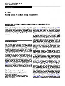
The facility used for the current experiments is shown in figure 1. A stationary target was mounted on a vibration-free frame and placed in the tank at two locations (mid-width (19.7 cm) and full-width (39 cm)) (figure 2). The placement of the target determined the path length Lp of the light from through the stratified fluid. The target was centered vertically in the tank, where the stratification remained constant throughout the experiment. The facility was stably stratified with a linear salinity distribution using the standard double-bucket method (Fortuin 1960). Following stratification, initial temperature and salinity profiles were measured with a temperature-conductivity probe and density profiles and the buoyancy frequency N = − g ρ 0 dρ dz were computed. The reference density ρ0 is taken to be the density at mid-depth.
Pulley
Connecting rod
Combs
Rack
Motor Flywheel
Electrical box
Enclosure Test section
Rods
Window
Supports
Figure 1. Experimental facility Turbulence was generated using a grid of horizontally oscillating vertical rods with a constant stroke length S of 7.5 cm and frequency ω. To reduce mean flows, neighboring combs (10 total) oscillated 180 degrees out of phase. During the stirring,
3
the force on one of the rods was measured using a small load cell so that the work done by the rods on the fluid could be estimated. Also, the temperature-conductivity probe was placed at mid-depth and sampled continuously during stirring to obtain scalar and density fluctuations. Sequential images of the stationary target separated by a time ∆t were taken using a TSI model 630044 Cross Correlation CCD camera and TSI model 600066 frame grabber board. The host computer was a Dell Optiplex 300 MHz running Windows NT. Typically, ∆t is chosen so that particles will not leave the interrogation window between two images in a pair. However, since the particles in our experiment have no mean motion, we chose ∆t = 0.05 seconds, which gave the maximum apparent particle displacements in preliminary experiments. This choice was then evaluated by performing a sensitivity analysis of ∆t with the gathered data as well as comparing with the integral timescale obtained from the density fluctuations during stirring. The results of this analysis will be discussed in the results section. Approximately 32 image pairs were captured for each stirring intensity. The images were processed using a straddled cross correlation algorithm with a centroid peak search and a 64 x 64 pixel interrogation area. The field of view was approximately 5 cm x 5 cm. For presentation, the 32 rms velocity fields were ensemble averaged and then spatially averaged to provide a representative velocity error in the horizontal and in the vertical for each intensity. Full-width mount
Mid-width mount Vibration-free frame
Stationary Target
PC
CCD Camera Stirring Rod Continuous Illumination
Lp
Figure 2. Experimental setup (cross section) Following each stirring cycle, the motions were allowed to decay for a sufficient period, and profiles were again measured. The scalar profiles were then used to compute density profiles, from which the potential energy PE can be computed. The
4
change in the potential energy was then computed over the stirring cycle. The energy budget for these experiments is dW dPE = + ∫ ρ 0 εdV , dt dt V
(1)
which states that the rate of change of work W is equal to the rate of change of potential energy plus the dissipation ε integrated over the fluid volume V. The volume-averaged dissipation can be computed as
εa =
1 dW dPE ( − ). ρ 0V dt dt
(2)
With an estimate of the dissipation, the parameter εa/νN2 can be calculated for each of the experiments. This parameter, used often in oceanographic measurements, can be related to the intensity of the turbulence in a stratified flow. Higher εa/νN2 corresponds to higher turbulence intensities. Five turbulence intensities were tested at both the mid-width and full-width target positions. Subsequent experiments were performed using different initial stratifications. Table 1 contains the experimental details. Table1. Experimental parameters Expt No 2 4 5 6
ω (rad/s) 0.497 – 4.29 0.556 – 4.28 0.499 – 4.28 0.528 – 4.29
Lp (cm) 39.0 19.7 19.7 39.0
∆t (s) N (rad/s) 0.05 0.05 0.05 0.05
0.511 0.513 0.442 0.435
εa/νN2 34 - 17000 38 - 15500 42 - 23600 54 - 26500
RESULTS
Since the results of this analysis depend on the chosen value of ∆t, we analyzed the effect of ∆t on the results. Images gathered at a ∆t of 0.05 seconds were cross correlated with one another in a manner that varied ∆t over 0.05 to 0.45 seconds. The results were ensemble averaged for two of the five turbulence intensities for experiment 4. In both cases the velocity error increases from 0.05 to 0.13 seconds and then decreases from 0.13 to 0.45 seconds. This result suggests that the maximum velocity error occurs for a ∆t of 0.13 seconds. The rms velocity errors are approximately 60% higher for ∆t = 0.13 seconds than for ∆t = 0.05 seconds. The latter value was used in the following analysis. Figure 3 shows the rms fluctuations in horizontal velocity u and vertical velocity w as a function of the stirring frequency for two path lengths and two strengths of stratification. The rms velocities increase with increasing stirring intensity for both path
5
lengths: More energetic turbulence results in greater fluctuations in the index of refraction since it can lift blobs of dense fluid higher into the lighter fluid above. The velocity errors are quite small and arguably negligible compared to typical mean flows. The velocity errors in the horizontal are an order of magnitude greater that those in the vertical because of the anisotropy of the refractive index field generated by the stratified turbulence.
Figure 3. RMS velocity errors as a function of stirring frequency. Squares correspond to Lp = 19.7 cm while circles correspond to Lp = 39 cm. Closed symbols are for N = 0.4 and open symbols are for N = 0.5 rad/s. The rms velocity errors also depend on the buoyancy frequency N and the length Lp of the path through the variable refractive index field. The buoyancy frequency has little effect on the results from the shorter path but significantly changes the results for the longer path: The rms velocity errors almost double for all stirring frequencies when the buoyancy frequency is increased from 0.43 to 0.51 rad/s. Effects of the path length are unclear. Work of McDougall (1979) can be extended to predict that the rms displacement of a beam of light should increase as L3p/ 2 . However, the rms horizontal velocity error for the longer path case exceeds that for the shorter path only for high buoyancy frequency and low stirring frequency. In all other cases, the rms velocity errors are smaller for higher Lp. The increase in the path length
6
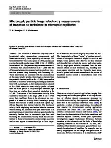
may cause the deviations of the light to average out to the mean position, the position of the particle. Also, for the longer path, the particle images are quite blurred (figure 4); future work includes determining the effect of the blurring on the PIV algorithm and using strobe lighting instead of continuous lighting to see whether blurring is reduced.
A
B
C
Figure 4. Images from experiments 4 (top) and 6 (bottom). Lp is 19.7 cm for experiment 4 and 39 cm for experiment 6. Low, medium, and high stirring intensities correspond to A, B, and C, respectively. To make the results of these experiments more generally applicable, we present the results in nondimensional form. We parameterize the rms velocity error by εa/νN2 and normalize the rms velocity error by the velocity scale Sω of the stirring. Figure 5 shows the normalized rms velocity errors as functions of εa/νN2. Once again, the results are plotted for two different path lengths and two stratification strengths. The rms velocity errors are small compared to the forcing, and the horizontal errors are several times the magnitude of the vertical velocity errors. We plan to measure the rms velocity fluctuations in an unstratified fluid using a full PIV setup to provide a better means of normalizing the velocity error, but for now we use the results of Hopfinger and Toly (1976) for turbulence generated by a vertically oscillated grid to estimate the rms velocity due to the stirring rods in our tank. Hopfinger and Toly found u rms C 1 / 2 1 / 2 −1 = S M z Sω 2π
7
(3)
where C is taken to be 0.3, M is the transverse bar spacing (4 cm), and z is the virtual origin taken to be half the longitudinal bar spacing (7.5 cm). For the stroke length and stirring frequencies used in these experiments, we find urms/Sω = 0.04. The measured rms velocity error is at most 5% of this value suggesting that the rms velocity error is negligible at this value of ∆t. The errors now decrease with increasing turbulence intensity since Sω grows faster than the errors. One would expect the error to go to zero for no stratification ) and for no stirring (εa/νN2 0). Our velocity errors appear to approach (εa/νN2 zero for large εa/νN2, but no tendency toward zero for small εa/νN2 can be discerned. Like figure 3, figure 5 shows the initial stratification strength has more of an effect on the higher path length experiments; however, for both horizontal and vertical velocity errors the effect of the stratification strength diminishes with increasing turbulence intensity. Finally, the path length seems to have less of an effect in this nondimensional form, but effects of the blurring of the images in the longer path case at medium to high intensities (εa/νN2 > 1000) remain to be determined.
→∞
→
Figure 5. Normalized rms velocity errors as a function of turbulence intensity. Squares correspond to Lp = 19.7 cm while circles correspond to Lp = 39 cm. Closed symbols are for N = 0.4 and open symbols are for N = 0.5 rad/s.
8
Conclusions and Future Work
Experiments were performed to evaluate the error in velocity measurements made using PIV in a stratified flow with a fluctuating refractive index field. Errors were evaluated by imaging a stationary target resembling a typical PIV image through a stratified, turbulent flow. We find apparent velocities recorded by the PIV system to be small compared to the rms velocities induced by the stirring rods. The maximum rms velocity errors are only approximately 8% of the estimated grid induced rms velocities. Future work will measure the true grid induced rms velocities using PIV in an unstratified system allowing a more accurate comparison of the magnitude of these errors. We will also investigate the effects of image blurring on the PIV algorithm as well as perform pulsed rather than continuous illumination experiments with hopes of reducing the blurring at high turbulence intensities and long path lengths. REFERENCES
Alahyari, A. and Longmire, E.K. (1994), Particle image velocimetry in a variable density flow: Application to a dynamically evolving microburst. Exp. Fluids, 17, 434-440. Barrett, T.K. and Van Atta, C.W. (1991), Experiments on the inhibition of mixing in stably stratified decaying turbulence using laser Doppler anemometry and laser-induced fluorescence. Phys. Fluids A, 3, 1321-1332. Fernandes, R.L.J. 2001 The spatial structure of turbulent Rayleigh-Benard Convection. PhD Thesis, University of Illinois at Urbana-Champaign. Fincham, A.M., Maxworthy, T., and Spedding, G.R. (1996), Energy dissipation and vortex structure in a freely decaying, stratified grid turbulence. Dyn. Atmos. Ocean, 23,155-169. Fincham, A.M. and Spedding, G.R. (1997), Low cost, high resolution DPIV measurement of turbulent fluid flow. Exp. Fluids, 23, 449-462. Fortuin, J. 1960: Theory and application of two supplementary methods of constructing density gradient columns. J. Polymer Sci., 44, 505–515. Hannoun, I.A., Fernando, H.J.S., and List, E.J. (1988), Turbulence structure near a sharp density interface. J. Fluid Mech., 189, 189-209. Hopfinger, E.J. and Toly, J.A. (1976), Spatially decaying turbulence and its relation to mixing across density interfaces. J. Fluid Mech., 78, 155-175. McDougall, T.J. (1979), On the elimination of refractive index variations in turbulent density-stratified liquid flows. J. Fluid Mech., 93, 83-96. Nimmo Smith, W.A., Luznik, L., Katz, J., and Osborn, T.R. (2002), Flow structure and turbulence distributions in the coastal ocean from PIV data. 2002 Ocean Sciences Meeting, Honolulu. Spedding, G.R., Browand, F.K., and Fincham, A.M. (1996), The long-time evolution of the initially turbulent wake of a sphere in a stable stratification. Dyn. Atmos. Ocean, 23,171-182. Spedding, G.R. (1997), The evolution of initially turbulent bluff-body wakes at high internal Froude number. J. Fluid Mech., 337, 283-301.
9