Jul 12, 2016 - method for Higgs-boson production in gluonâgluon fusion are elaborated, including also ... from Feynman diagrams, but deduced from PDF momentum sum rules. .... In the following we shall elaborate mainly on the hadronâhadron collision producing the .... 5This is, of course, not true for other processes.
IFJPAN-IV-2016-9 CERN-TH-2016-132 MCnet-16-18
arXiv:1606.00355v2 [hep-ph] 12 Jul 2016
Parton distribution functions in Monte Carlo factorisation scheme? S. Jadacha , W. Placzekb , S. Sapetac,a , A. Si´odmokc,a and M. Skrzypeka a
Institute of Nuclear Physics, Polish Academy of Sciences, ul. Radzikowskiego 152, 31-342 Krak´ow, Poland b Marian Smoluchowski Institute of Physics, Jagiellonian University, ul. Lojasiewicza 11, 30-348 Krak´ow, Poland c Theoretical Physics Department, CERN, Geneva, Switzerland
Abstract A next step in development of the KrkNLO method of including complete NLO QCD corrections to hard processes in a LO parton-shower Monte Carlo (PSMC) is presented. It consists of generalisation of the method, previously used for the Drell–Yan process, to Higgs-boson production. This extension is accompanied with the complete description of parton distribution functions (PDFs) in a dedicated, Monte Carlo (MC) factorisation scheme, applicable to any process of production of one or more colour-neutral particles in hadron–hadron collisions.
?
This work is partly supported by the Polish National Science Center grant DEC-2011/03/B/ST2/02632 and the Polish National Science Centre grant UMO-2012/04/M/ST2/00240.
1
Introduction
The method of including complete NLO QCD corrections to hard processes in the LO parton-shower Monte Carlo (PSMC), nicknamed KrkNLO, was originally proposed in Ref. [1], where its first numerical implementation on top of a toy-model PSMC was also presented. It was restricted there to gluon emission only and was elaborated for two processes: Z/γ ∗ production in hadron–hadron collisions, i.e. the Drell–Yan (DY) process and deep inelastic electron–hadron scattering (DIS). In the following Ref. [2], the KrkNLO method was implemented for Z/γ ∗ production process at large hadron collider (LHC) in combination with Sherpa [3] and Herwig++ [4– 6] PSMCs. Many NLO-class numerical results (distributions of transverse momenta, rapidity, integrated cross sections, etc.) were presented there and comparisons of the KrkNLO predictions with those from other methods, such as MC@NLO [7] and POWHEG [8], were also performed. The main advantage of the KrkNLO method with respect to other, older methods of matching the fixed-order NLO calculations with PSMCs (MC@NLO and POWHEG ) is its simplicity. This simplicity stems from the fact that the entire NLO corrections are implemented using a simple positive multiplicative MC weight. However, in order to profit from it, one has to use in the KrkNLO method parton distribution functions (PDFs) in a special, so-called Monte Carlo (MC) factorisation scheme and PSMC has to fulfil some minimum quality criteria. Most of modern PSMCs are good enough for the KrkNLO method. Construction of PDFs in the MC factorisation scheme (FS) has evolved step by step: in Ref. [1] it was defined for gluonstrahlung only (albeit for two different processes, DY and DIS). In Ref. [2], the KrkNLO PDFs in the MC FS were defined and numerically constructed including also gluon to quark transitions/splittings, relevant for the complete NLO corrections in the DY process, which at the LO level has only quarks and antiquarks in the initial state. PDFs in the MC scheme in Ref. [2] were defined in terms of the standard MS PDFs, and constructed numerically by transforming the MS PDFs into MC-scheme PDFs, before they were plugged into PSMC used in the KrkNLO method. However, in Ref. [2] certain elements in the transition matrix K, transforming the MS PDFs into the MC-scheme PDFs could be omitted, because they were not relevant (i.e. of a NNLO class) for the DY process. These elements of the transition matrix have to be added for any process with initial-state gluons, such as the Higgs-boson production elaborated in the present work. They will be defined and applied in the following, such that the complete transition matrix K transforming the MS PDFs into the MC-scheme PDFs will be specified for the first time. It will be argued that PDFs in such a MCscheme can serve in the KrkNLO method for any process at a hadron–hadron collider in which a colour-neutral single or multiple system of heavy particles is produced. For other processes, with one or more coloured partons in the final state at LO level, the KrkNLO method with PDFs in the MC scheme may also work, but this subject is reserved for the forthcoming publications. The MC factorisation scheme is a complete scheme, such that NLO coefficient functions 1
for any hard process under consideration are known, hence PDFs in the MC FS can be fitted directly to experimental DIS and DY data. However, at present, we obtain them from PDFs in the MS scheme and leave out direct fitting to data for the future developments. On the methodological side, as seen in Refs. [1, 2], the essence of the KrkNLO method is that certain NLO correction terms in an unintegrated/exclusive form present in the MS scheme, which are proportional to unphysical Dirac-delta terms in transverse momentum of emitted real partons, are removed in the KrkNLO methodology by means of redefinition of PDFs from the MS to MC scheme. These ‘pathological’ terms are preventing the use of a simple multiplicative MC weight for implementing NLO corrections in the MS scheme in real-emission phase space, and they complicate implementation of the MC@NLO and POWHEG methods. These peculiar terms can be determined and calculated either by means of studying the NLO corrections to hard process (coefficient functions), or, alternatively, by means of integrating soft-collinear counter terms (similar to these in the Catani–Seymour method [9]), which define the MC-scheme PDFs in d = 4 + 2ε dimensions1 . We are going to calculate them using both methods, obtaining the same results. Last but not least, the NLO calculations for the DY process of Ref. [2] were also compared with NNLO calculations, concluding that they are closer to the latter than the results of the MC@NLO and POWHEG methods. The outline of the paper is the following: in Section 2 the KrkNLO method is characterised briefly. In Section 3 all distributions needed for implementation of the KrkNLO method for Higgs-boson production in gluon–gluon fusion are elaborated, including also many analytical crosschecks and a necessary update of the virtual corrections in softcollinear counter terms used in Ref. [2] for the Z/γ ∗ (DY) process. Section 4 presents numerical results for PDFs in the MC scheme. Then, first numerical results for the total cross section from the KrkNLO method for the Higgs production at the LHC are shown in Section 5. Finally, in Section 6 we summarise the paper and discuss future prospects of our work.
2
The method
The KrkNLO method was formulated in a few variants. For instance, in the version of Ref. [1], the MC weight implementing the NLO corrections sums the contributions from all relevant partons generated in PSMC next to the hard process “democratically”, such that it works equally well for PSMCs based on angular ordering or virtuality ordering, contrary to POWHEG which requires adding extra gluons to a PSMC event. In the present work, we are going to follow the variant of KrkNLO discussed in Ref. [2], in which the NLO-correcting MC weight uses only one parton, the one closest to the hard process in the transverse momentum, that is the 1st parton generated in the backward evolution (BEV) in the PSMC algorithm with kT -ordering. 1
They also form matrix elements of the K-matrix transforming PDFs from the MS to MC scheme.
2
In any case, in the KrkNLO method, the entire event of PSMC is preserved and reweighted, contrary to POWHEG and MC@NLO where the parton attributed to the hard process is generated outside PSMC and, only later on, the remaining partons are provided by PSMC. Obviously, this puts certain minimum quality requirements on the the PSMC: (i) the 1st parton in BEV algorithm has to be generated with the distribution which has a correct soft and collinear limit and (ii) its phase space in momentum and flavour space has to be covered completely, without empty regions. Luckily, the above requirement is fulfilled by all modern PSMCs for initial-state emissions discussed in this work. It is worth to comment in advance on the apparent use in the following of the softcollinear counter terms (dipoles) of the Catani–Seymour (CS) subtraction scheme [9]. Their role is two-fold: (1) the CS dipoles serve us as a useful benchmark, as they provide a reference model for QCD distributions of real emissions featuring the exact soft and collinear limits and (2) the CS scheme helps us in a proper inclusion of the NLO virtual corrections. However, let us point out immediately an important difference between the MC and CS scheme: the CS dipoles do not include virtual corrections, while softcollinear counter terms (SCCTs) of the KrkNLO do include them, albeit not calculated from Feynman diagrams, but deduced from PDF momentum sum rules. The role of the SCCTs in the KrkNLO methodology is also much richer than that of the dipoles in the CS scheme – our SCCTs not only provide subtractions of soft-collinear singularities in real-emission phase space, but they are also used to define PDFs in the MC factorisation scheme. Moreover, their sums are required to coincide with the corresponding sums of real-parton distributions in PSMC2 .
3
Higgs production in gluon–gluon fusion
In the following we are going to collect all distributions needed for implementation of the KrkNLO method for the gluon-fusion Higgs production in hadron–hadron collisions. Elements of the matrix transforming PDFs from the MS to MC scheme will be also obtained as a byproduct. We start necessarily from the leading order (LO) process g(p1 ) + g(p2 ) −→ H(Q) ,
(3.1)
see Fig. 1, where Q = p1 + p2 . The LO matrix element squared, in the limit mt → ∞ and neglecting all other quarks contributions, reads 2 |MLO gg | =
αs2 Q4 , 2 2 576π v
2
(3.2)
At least for the initial-state emitters in the present work, but also in the final-state ones in the future implementations of the KrkNLO method. In fact, SCCTs of the KrkNLO and PSMC distributions do not need to coincide exactly, but optional additional weight bringing the PSMC to SCCT distribution of the KrkNLO method has to be well behaved.
3
Figure 1: The LO Feynman diagram for the process of Higgs boson production in gluon–gluon fusion. The effective vertex (black dot) corresponds to a quark loop with summation over all quarks, in which the top-quark mass is set to infinity while the masses of the other quarks are set to zero. √ where v 2 = ( 2GF )−1 is the Higgs vacuum expectation value (VEV) squared. Hence, the LO total cross section takes the form LO σ0 ≡ σgg (Q2 ) =
π αs2 LO 2 |M | = . gg Q4 576πv 2
(3.3)
For all NLO subprocesses (channels) a(p1 ) + b(p2 ) −→ H(Q) + c(k),
(3.4)
where a and b are incoming partons (gluons and/or quarks), while c is an outgoing parton (quark or gluon) we shall use the same parametrisation of the kinematics in terms of the following Sudakov variables: α=
p2 · k , p1 · p2
β=
p1 · k , p1 · p2
α + β = 1 − z ≤ 1.
(3.5)
For the gg-channel NLO subprocess g + g −→ H + g ,
(3.6)
shown in Fig. 2, the matrix element squared reads 2 |MNLO gg | = 8παs CA
1 1 + z 4 + α4 + β 4 2 |MLO gg | . zQ2 αβ
(3.7)
For the qg-channel NLO subprocess g + q −→ H + q ,
(3.8)
shown in Fig. 3, one obtains 2 |MNLO gq | = 8παs CF
1 1 + β2 2 |MLO gg | , 2 zQ α 4
(3.9)
Figure 2: The NLO Feynman diagrams for real-parton radiation in the process of Higgs-boson production in gluon–gluon fusion: the gg channel.
Figure 3: The NLO Feynman diagram for real-parton radiation in the process of Higgs-boson production in gluon–gluon fusion: the gq channel.
Figure 4: The NLO Feynman diagram for real-parton radiation in the process of Higgs-boson production in gluon–gluon fusion: the q q¯ channel. Finally, for the q q¯ channel q + q¯ −→ H + g ,
5
(3.10)
see Fig. 4, one has 2 |MNLO q q¯ | = 8παs CF
� 8 1 2 2 2 |MLO α + β gg | . 2 3 zQ
(3.11)
This last process, unlike the previous ones, is not generated by the backward-evolution PSMC starting from the gg → H hard process, hence in the KrkNLO method, its contribution cannot be treated by NLO-reweighting of events generated by the main branch of the LO PSMC algorithm. It has to be added as an extra tree-level LO process to PSMC. Moreover, it is free of collinear and soft singularities. This poses no problem as most of present-day PSMCs implement such a process.
3.1
CS dipoles and MC matrix elements
In the following we shall elaborate mainly on the hadron–hadron collision producing the Higgs boson or Z/γ ∗ (Drell–Yan process). However, components of the KrkNLO method defined here will be also applicable to any LO process a + a ¯ → X and the corresponding ± + − a + b → X + c where X = H, Z/γ, W , ZZ, W W or any other colour-neutral heavy object; a, b = q, q¯, g are initial coloured partons and c is an additional parton emitted at the NLO level.
Figure 5: Kinematics of a single channel with one CS splitting. In the following formulation of the KrkNLO-method components, the CS dipoles will serve us as useful auxiliary objects. They are formed by an initial-state (on-shell) emitter a from one hadron and a spectator parton b from another hadron3 , see Fig. 5. Following closely the notation of the CS work [9], the emitter a splits into an off-shell ac e = ¯b (ac,b) entering into the hard process and an emitted parton c. The CS dipoles D relevant ¯ for processes of our interest are proportional to Pac,a e e , the DGLAP kernel for the a → ac splitting4 . 3 4
The role of the spectator is to provide for momentum and colour conservation. In the case of the emitted parton c being the gluon one gets ac e ≡ a.
6
a+b→c+H
a + b → c + Z/γ
(a, b)
(ac, b)
(a, b)
(ac, b)
(g, g)
(gg, g)
(q, q¯)
(qg, q¯)
(q, g)
(qq, g)
(¯ q , q)
(¯ q g, q)
(¯ q , g)
(¯ q q¯, g)
(g, q)
(gq, q)
(g, q¯)
(g q¯, q¯)
Table 1: List of indices labelling the CS or MC soft-collinear counter terms for all the NLO channels (except the q q¯ channel in Higgs production) of annihilation processes. Indices (a, b) denote initial partons (channel), while (ac, b) are labelling the CS/MC counter terms, with a being an emitter and b a spectator. For the processes of the annihilation a¯ a → X at the LO level, such as the Higgs production and the DY process, in each NLO channel ab → cX we must have ac e = ¯b in the NLO splitting. In other words, the NLO splitting in the annihilation processes is fully determined by a and b5 . The above rules are illustrated in Fig. 5 and possible indices are listed in Table 1 for the emission from the incoming line a6 . Let us first define explicitly the MC distributions (matrix elements) and the CS dipoles representing the initial-state real-parton emissions for the Higgs production process in d = 4 + 2ε dimensions: (A) For the g + g → H + g channel a typical/representative distribution of PSMC, summing the emissions from both incoming gluons, is 2 −2� |MMC gg→Hg | = 8παs µ
1 1 2 (1 − z)Pˆgg (z; �)|MLO gg→H | , Q2 αβ
where the g → g splitting function is given by � � z 1 − z 1 + z 4 + (1 − z)4 ˆ Pgg (z; �) = 2CA + + z(1 − z) = CA . 1−z z z(1 − z) (gg,g)
2 It is equal to the sum of two CS dipoles |MMC gg→Hg | = D(1) (gg,g)
D(1)
=
α 2 |MMC gg→Hg | , α+β
(gg,g)
D(2)
=
(3.12)
(3.13)
(gg,g)
+ D(2) , where
β 2 |MMC gg→Hg | , α+β
(3.14)
β α with soft partition functions α+β and α+β separating the soft singularity evenly between two incoming emitters. Indices (1) and (2) are used to distinguish the above two dipoles. 5 6
This is, of course, not true for other processes. Rules for emissions from the second incoming line are analogous.
7
(B) For the g + q → H + q channel we have (with a single soft-collinear pole the softpartition functions are not needed): (qq,g)
2 |MMC gq→Hq | = D(1)
= 8παs µ−2�
1 1 ˆ 2 Pgq (z; �)|MLO gg→H | , 2 Q α
where the q → g splitting function reads � � 2 1 + (1 − z) + �z . Pˆgq (z; �) = CF z
(3.15)
(3.16)
(C) Finally, for the g + q¯ → H + q¯ channel, the CS dipole and MC distribution is the same as the previous one for quarks. The above distributions agree with these used in the POWHEG-method construction of Ref. [10]. For the sake of completeness, let us collect the CS dipoles and MC distributions already known from Refs. [1, 2], with the q → q and g → q splittings. They will be needed in the following to define the transition matrix K from the MS to MC factorisation scheme for all PDFs. (A) For the q + q¯ → Z + g channel, the MC distribution reads: (qg,¯ q)
2 |MMC q q¯→Zg | = D(1)
where
(¯ q g,q)
+ D(2)
= 8παs µ−2�
1 1 2 (1 − z)Pˆqq (z; �)|MLO q q¯→Z | , (3.17) Q2 αβ
� � 1 + z2 ˆ Pqq (z; �) = CF + �(1 − z) , 1−z
(3.18)
and the soft-partition function is used again: (qg,¯ q)
D(1)
=
α 2 |MMC q q¯→Zg | , α+β
(¯ q g,q)
D(2)
=
β 2 |MMC q q¯→Zg | . α+β
(3.19)
(B) For the q + g → Z + q channel we have (the soft partition function in the MC distribution is not necessary): (gq,q)
2 |MMC qg→Zq | = D(1)
= 8παs µ−2�
1 1 ˆ 2 Pqg (z; �)|MLO q q¯→Z | , 2 Q α
(3.20)
where � � Pˆqg (z; �) = TR z 2 + (1 − z)2 + 2� z(1 − z) .
(3.21)
It should be stressed that all the above MC distributions and CS dipoles are basically in the exclusive (unintegrated) form.
8
All the above relations between the MC distributions and the exclusive MC/CS counter terms for any annihilation processes can be summarised in a compact formula as follows: (ac,b)
2 |MMC ab→cX | = D(1)
(bc,a)
+ D(2) ,
(3.22)
where translation from the indices (ab) to (abc) is unique for a given annihilation process and for a given initial parton splitting, as demonstrated explicitly in Table 1 for the splitting of the initial parton a, see also Fig. 5. Moreover, on the RHS of the above relation only one of D’s is nonzero, except for the c = g case (gluonstrahlung), but in this case both D’s are equal. Hence, there is in practice one-to-one correspondence (ab) ↔ (abc) for all annihilation processes, to be often exploited in the following section.
3.2
Integrated CS dipoles and counter terms of MC scheme
For the purpose of installing virtual parts (using PDF momentum sum rules) in the MC distributions (soft-collinear counter terms) and defining the K-matrix for transforming PDFs from the MS to MC scheme, we need to integrate partly all distributions defined in the previous subsection, keeping the z = 1 − α − β variable fixed. A z-dependent differential cross section corresponding to the real-emission MC matrix elements can be expressed in the following way: Z MC σab,R (z, �) 1 1 dˆ 2 ˆ ˆ MC = |MMC (3.23) ab→Xc | dΦ = σ0 Γab,R (z, �), z dz 2Q2 MC where Γˆab,R (z, �) is the MC real-emission function corresponding to the partly integrated MC distribution of the previous subsection for a given process: a + b → X + c. The integration element dΦˆ can be expressed in terms of the Sudakov variables as follows � �−� 1 4π 1 ˆ dΦ = (αβ)� δ(1−z−α−β)θ(α)θ(1−α)θ(β)θ(1−β)θ(1−α−β) dα dβ . 8π s Γ (1 + �) (3.24) The above expressions are defined in d = 4 + 2� dimensions in order to regularise, in the usual way, the soft and collinear singularities of the real-parton radiation. Using the exact NLO matrix element, one can similarly write, for each channel ab, a regularised partly integrated NLO cross section for real-parton emission: Z NLO σab,R (z, �) 1 dˆ 1 2 ˆ (3.25) = |MNLO ˆNLO ab→Xc,R | dΦ = σ0 ρ ab,R (z, �). 2 z dz 2Q
Following the relation of Eq. (3.22), one may also define the relation of the integrated MC distribution to the individual integrated soft-collinear counter terms: MC Γˆab,R (z, �) = ΛˆMC (z, �) + ΛˆMC (z, �) e (ac,b),R e (bc,a),R
(3.26)
R where ΛˆR are the corresponding integrals dΦˆ D as in Eq. (3.23). However, contrary to the CS counter terms, the counter terms ΛˆMC of the MC scheme (and the Γˆ MC radiation 9
functions as well) will also include virtual corrections, calculated using the momentum sum rules, see next subsections for details. Let us calculate all the above objects with more details for the gg → Hg channel and then, skipping details of analytical integration, for other channels.
3.3
gg → Hg channel
A real-emission part of the MC radiation function results from the following integration7 � � Z 2 −� 1 4πµ 1 2C α 1 A s MC 2 MC ˆ= |M | d Φ Γˆgg,R (z, �) = gg→Hg σ0 2Q2 2π s Γ (1 + �) � �Z 1 Z 1 2 (1 − z) (3.27) × z+ + z(1 − z)2 dα dβ (αβ)−1+� δ1−z=α+β z 0 0 � �−� � � αs 4πµ2 Γ (1 + �) −� (1 − z)2 −1+2� 2 2 = 2CA z (1 − z) + z(1 − z) . z+ 2π Q2 Γ (1 + 2�) � z Using the standard expansion (1 − z)−1+2� =
1 δ(1 − z) + 2�
� ln(1−z) � 1 + 2� 1−z + 1−z +
we obtain
( � � � �� � 2 −� 2C α 2 4πµ Γ (1 + �) δ(1 − z) 1 1 A s MC Γˆgg,R (z, �) = + + − 2 + z(1 − z) 2π Q2 Γ (1 + 2�) �2 � 1−z + z ) � � � � � �� � 1 ln(1 − z) 1 1 +4 − [2 − z(1 − z)] ln(1 − z) − 2 + − 2 + z(1 − z) ln z . z 1−z 1−z + z + (3.28) The NLO real correction according to Ref. [11] reads ( � � �−� �� � 2CA αs 4πµ2 Γ (1 + �) δ(1 − z) 2 1 1 NLO ρˆgg,R (z, �) = + + − 2 + z(1 − z) 2π Q2 Γ (1 + 2�) �2 � 1−z + z � � � � 1 ln(1 − z) +4 − [2 − z(1 − z)] ln(1 − z) z 1−z + ) � � �� 1 11 (1 − z)3 1 −2 + − 2 + z(1 − z) ln z − . 1−z + z 6 z (3.29) From the above equations we readily obtain the NLO real coefficient function in the MC scheme: � � 3 α 11 (1 − z) s MC NLO MC Hgg,R (z) = ρˆgg,R (z, �) − Γˆgg,R (z, �) = 2CA − . (3.30) 2π 6 z 7
We employ here and in the following a shorthand notation δx=y ≡ δ(x − y).
10
The same expression is obtained in 4 dimensions by means of performing first the MCdipole subtraction and then integrating the finite result over the phase space: Z � � NLO 2 2CA αs 1 1 1 MC MC 2 Hgg,R (z) = dΦ = |M | − |M | gg gg→Hg σ0 2Q2 2π 2z Z 1 Z 1 4 4 4 2 1 + z + α + β − 2[z + (1 − z)2 + z 2 (1 − z)2 ] dα dβ δ1−z=α+β × (3.31) αβ 0 � 0 � 11 (1 − z)3 αs 2CA − . = 2π 6 z A virtual correction to the above MC radiation function Γˆgg is calculated from the momentum sum rules: Z 1 h i MC MC MC ˆ Γgg,V (z, �) = −δ(1 − z) dz z Γˆgg,R (z, �) + 2nf · 2Γˆqg (z, �) , (3.32) 0
where nf is the number of fermions. The first part in the above virtual correction resulting from integration over the first term in brackets on RHS reads as follows: Z 1 MC MC ˆ dz z Γˆgg,R (z, �) Γgg,V1 (z, �) = −δ(1 − z) 0 (3.33) � � � �−� αs 1 11 1 341 π 2 4πµ2 Γ (1 + �) = δ(1 − z) 2CA − 2+ − − . 2π Q2 Γ (1 + 2�) � 6 � 72 3 In order to calculate the second part to the virtual correction in RHS of Eq. (3.32) we need to know first the following MC radiation functions for the g → q transition, e.g. from the process q + g → Z + q: � � Z 2 −� 1 4πµ Γ (1 + �) α 1 s MC MC 2 |Mqg→Zq | dΦˆ = TR Γˆqg (z, �) = 2 2 σ0 2Q 2π Q Γ (1 + 2�) ( ) (3.34) � � 2 � (1 − z)2 1� 2 2 2 × z + (1 − z) + z + (1 − z) ln + 2z(1 − z) + O(ε) , � z 2 where |MMC qg→Zq | is shown in Eq. (3.20). Using the above result we can cross-check the formula for the gluon-channel MC radiation function of the DY process calculated previously in 4 dimensions in Ref. [2]. For the exact NLO contribution Ref. [12] provides
ρˆNLO qg→Zq (z, �) ( ×
αs = TR 2π
�
4πµ2 Q2
�−�
Γ (1 + �) Γ (1 + 2�)
) 2 � � � 1� 2 (1 − z) 7 1 z + (1 − z)2 + z 2 + (1 − z)2 ln − z 2 + 3z + . � z 2 2
11
(3.35)
Then, the resulting coefficient function for the DY process in the MC scheme reads � � αs 1 MC NLO MC ˆ Cqg (z) = ρˆqg→Zq (z, �) − Γqg (z, �) = TR (1 − z)(1 + 3z) , (3.36) 2π 2 which agrees with our previous result, given in Ref. [2]. For the sake of completeness, the corresponding coefficient function in the MS factorisation scheme reads: � � � 2 � (1 − z)2 7 2 1 αs 2 MS TR z + (1 − z) ln − z + 3z + (3.37) Cqg (z) = 2π z 2 2 and the transition matrix element transforming part of gluon MS PDF into the quark PDF in the MC scheme is given by � � � 2 � (1 − z)2 αs MS MC 2 MC TR z + (1 − z) ln + 2z(1 − z) . (3.38) Kqg (z) = Cqg (z) − Cqg (z) = 2π z The above was obtained by comparing the NLO coefficient functions for the DY process in the MS and MC schemes. However, exactly the same result can be obtained alternatively from the difference of the soft-collinear counter terms in these two schemes: i h MS MC ˆ Kqg (z, �) , (3.39) (z) = ΛˆMC (z, �) − Λ qg qg �=0
where the universal MC-scheme counter term corresponding to the g → q transition is given by ˆ MC ΛˆMC (3.40) qg (z, �) = Γqg (z, �), MC where Γˆqg (z, �) is defined in Eq. (3.34), and the MS counter term is � �−� � 4πµ2 αs Γ (1 + �) 1 � 2 MS ˆ Λqg (z, �) = TR z + (1 − z)2 . 2 2π Q Γ (1 + 2�) �
(3.41)
After this brief detour to the DY process, we can now complete the calculation of the virtual correction to the MC radiation function for the gg → Hg channel. Using Eq. (3.34), the second term in RHS of Eq. (3.32) is calculated: Z 1 MC MC ˆ (z, �) Γgg,V2 (z, �) = −δ(1 − z) · 4nf dz z Γˆqg 0 (3.42) �−� � � � αs Γ (1 + �) 4πµ2 4 1 59 = δ(1 − z) nf TR − + . 2π Q2 Γ (1 + 2�) 3 � 18 The complete result for virtual correction to the gg → Hg MC radiation function, obtained from the momentum sum rule of Eq. (3.32), reads as follows: � � 2 −� 2C α 4πµ Γ (1 + �) A s MC MC MC Γˆgg,V (z, �) = Γˆgg,V1 (z, �) + Γˆgg,V2 (z, �) = δ(1 − z) 2π Q2 Γ (1 + 2�) ( ) (3.43) 2 1 1 11 − 4Tf /CA 341 π Tf 59 × − 2+ − − + , � � 6 72 3 CA 36 12
where Tf = nf TR . The complete MC radiation function for gg → Hg process is obtained finally in the following explicit form: � � 2 −� α 4πµ Γ (1 + �) s MC Γˆgg (z, �) = 2CA 2 2π Q Γ (1 + 2�) ( � � � � 2 11 − 4Tf /CA 1 1 × δ(1 − z) + + − 2 + z(1 − z) � 12 1−z + z (3.44) � � 2 341 Tf 59 π + − − δ(1 − z) 3 72 CA 36 ) � � � � ln(1 − z) 1 (1 − z)2 ln z +4 +2 − 2 + z(1 − z) ln −2 . 1−z + z z 1−z Let us also calculate the coefficient function in the MC scheme for the gg → Hg channel. Using the exact NLO virtual correction of Ref. [11]: � �−� 4πµ2 αs 2CA = δ(1 − z) 2π Q2 ( ) 1 1 11 − 4Tf /CA 11 π 2 11 − 4Tf /CA Q2 Γ (1 + �) − 2+ + + − ln 2 . Γ (1 + 2�) � � 6 6 3 6 µ
ρˆNLO gg,V (z, �)
(3.45)
we obtain the following virtual part of the coefficient function in the MC scheme (with the usual µ2 = Q2 assignment): � � 2 α 473 2π T 59 s f MC NLO MC Hgg,V (z) = ρˆgg,V (z, �) − Γˆgg,V (z, �) = 2CA δ(1 − z) + − . (3.46) 2π 72 3 CA 36 Combining the real and virtual contributions of Eqs. (3.30) and (3.46), the NLO coefficient function for the gg → Hg process in the MC factorisation scheme reads: � � � � αs 2 2 473 59 Tf 11 (1 − z)3 MC Hgg (z) = 2CA δ(1 − z) π + − − . (3.47) 2π 3 72 36 CA 6 z The analogous coefficient function in the MS factorisation scheme is obtained from Eqs. (3.29) and (3.45), after the standard subtraction of the MS soft-collinear counter terms (with µ2 = Q2 ) reads as follows: ( � 2 � � � α π 11 ln(1 − z) s MS Hgg (z) = 2CA δ(1 − z) + +4 2π 3 6 1−z + ) (3.48) � � 1 (1 − z)2 ln z 11 (1 − z)3 +2 − 2 + z(1 − z) ln −2 − . z z 1−z 6 z 13
With all the above results at hand we are also ready to determine the element g → g of the transition matrix for transforming PDFs from the MS to MC scheme: ( � 2 � h i α π 341 59 Tf 1 s MC MC MS Hgg (z) − Hgg (z) = CA − δ(1 − z) + − Kgg (z) = 2 2π 3 72 36 CA ) (3.49) � � � � ln(1 − z) 1 (1 − z)2 ln z 4 +2 − 2 + z(1 − z) ln −2 . 1−z + z z 1−z MC The same Kgg (z) it can be also obtained from the difference of the collinear counter terms: h i MC MS ˆ Kgg (z) = ΛˆMC (z, �) , (3.50) (z, �) − Λ gg gg �=0
ΛˆMC gg (z, �)
corresponding to the g → g transition where the universal MC counter term can be expressed in terms of the MC radiation function of Eq. (3.44) as follows 1 ˆ MC ΛˆMC gg (z, �) = Γgg (z, �), 2
(3.51)
and � �−� αs 4πµ2 Γ (1 + �) MS ˆ 2CA Λgg (z, �) = 2 2π Q Γ (1 + 2�) " # � � 11 − 4Tf /CA 1 1 1 + + − 2 + z(1 − z) × δ(1 − z) � 12 1−z + z
(3.52)
is the corresponding MS counter term.
3.4
gq → Hq channel
The channel g + q → H + q is easier because only real correction contributes at NLO. The corresponding MC radiation function can be readily obtained from the integral Z 1 1 2 ˆ MC ˆ Γgq (z, �) = |MMC gq→Hq | dΦ σ0 2Q2 � �−� � � � � (3.53) αs 4πµ2 Γ (1 + �) 1 + (1 − z)2 1 (1 − z)2 = CF + ln +z . 2π Q2 Γ (1 + 2�) z � z The exact NLO correction taken from Ref. [11] reads � �−� αs 4πµ2 Γ (1 + �) NLO ρˆgq (z, �) = CF 2π Q2 Γ (1 + 2�) ( ) � � 2 2 2 1 + (1 − z) 1 (1 − z) z − 6z + 3 × + ln − . z � z 2z 14
(3.54)
Combining the above two functions, the coefficient function for gq → Hq process in the MC factorisation scheme reads � � αs 3 (1 − z)2 MC NLO MC ˆ Hgq (z) = ρˆgq (z, �) − Γgq (z, �) = CF − . (3.55) 2π 2 z Exactly the same result can be obtained also from the following integral in 4 dimensions: Z � NLO 2 � 1 1 MC 2 Hgq (z) = |Mgq | − |MMC gq→Hq | dΦ 2 σ0 2Q Z Z 1 αs 1 1 1 + β 2 − [1 + (1 − z)2 ] = CF dα dβ δ(1 − z − α − β) (3.56) 2π z 0 α 0 � � αs 3 (1 − z)2 = CF − . 2π 2 z On the other hand, in the MS factorisation scheme (keeping µ2 = Q2 ), from Eq. (3.54) we can obtain (after the standard subtraction) the following coefficient function: � � αs 1 + (1 − z)2 (1 − z)2 z 2 − 6z + 3 MS CF ln − Hgq (z) = . (3.57) 2π z z 2z At this point we are able to define another element of the matrix transforming the MS gluon PDF into the gluon PDF of the MC-scheme � � αs 1 + (1 − z)2 (1 − z)2 MC MS MC Kgq (z) = Hgq (z) − Hgq (z) = CF ln +z . (3.58) 2π z z MC (z) can also be obtained from as a difference of the softAlternatively, the same Kgq collinear counter terms in the MC and MS schemes: h i MC MC MS ˆ ˆ Kgq (z) = Λgq (z, �) − Λgq (z, �) , (3.59) �=0
where, again, the universal MC-scheme counter term ΛˆMC gq (z, �) corresponding to the q → g MC transition can be related to the MC radiation function Γˆgq (z, �) of Eq. (3.53) as follows: ˆ MC ΛˆMC gq (z, �) = Γgq (z, �), and αs ΛˆMS CF gq (z, �) = 2π
�
4πµ2 Q2
�−�
Γ (1 + �) 1 1 + (1 − z)2 Γ (1 + 2�) � z
is the corresponding counter term in the MS scheme.
15
(3.60)
(3.61)
3.5
Revisiting q q¯ → Zg channel
In Ref. [2] the virtual correction to the MC counter term in the q q¯ channel was calculated from the quark-number conservation sum rule (as minus the integral over z of the real correction). This was justified for the DY process, for which the gluon PDF did not get corrected at NLO from the MS to MC factorisation scheme. Now, since we deal with the complete set of parton–parton transitions, including the transformation/correction of the gluon PDF, we have to rely on the momentum sum rule. For the pertinent channel this amounts to Z 1 h i MC ˆ ˆ MC (z, �) + Γˆ MC (z, �) . dz z ΓˆqMC Γqq¯,V (z, �) = −δ(1 − z) (z, �) + Γ (3.62) q¯,R gq g q¯ 0
Using the formula for the MC real-radiation function from Appendix B of Ref. [2]: ( � � 2 −� 2 1 + z2 4πµ Γ (1 + �) 2 α s C δ(1 − z) + ΓˆqMC (z, �) = F q¯,R 2π Q2 Γ (1 + 2�) �2 � (1 − z)+ ) (3.63) � � 2 ln(1 − z) 1 + z + 4(1 + z 2 ) −2 ln z + 2(1 − z) , 1−z + 1−z we can calculate the first part of the above virtual correction as follows: Z 1 MC ˆ dz z ΓˆqMC Γqq¯,V1 (z, �) = − δ(1 − z) q¯,R (z, �) 0 ( � � Z 1 2 −� 4πµ αs Γ (1 + �) 2 = − δ(1 − z) CF dz z δ(1 − z) 2 2π Q Γ (1 + 2�) 0 �2 ) (3.64) � � 2 2 ln(1 − z) 2 1+z 1+z + 4(1 + z 2 ) ln z + 2(1 − z) + −2 � (1 − z)+ 1−z + 1−z � �−� � � αs 4πµ2 Γ (1 + �) 2 17 1 163 2π 2 = δ(1 − z) CF − 2+ − − . 2π Q2 Γ (1 + 2�) � 3 � 18 3 For the second part, using Eq. (3.53), we obtain Z 1 i h MC MC ˆ (z, �) + ΓˆgMC (z, �) Γqq¯,V2 (z, �) = − δ(1 − z) dz z Γˆgq q¯ 0 � � −� αs 4πµ2 Γ (1 + �) = − 2 δ(1 − z) CF 2π Q2 Γ (1 + 2�) � � � � Z 1 � � 1 (1 − z)2 2 2 × dz 1 + (1 − z) + ln +z � z 0 � �−� � � αs 4πµ2 Γ (1 + �) 81 5 = δ(1 − z) CF − + . 2π Q2 Γ (1 + 2�) 3� 9 16
(3.65)
Thus the full virtual correction reads � �−� � � αs 4πµ2 2 Γ (1 + �) 3 17 2π 2 MC ˆ Γqq¯,V (z, �) = δ(1 − z) CF − 2+ − − . 2π Q2 Γ (1 + 2�) � � 2 3
(3.66)
After combining it with the real correction of Eq. (3.63) we obtain a complete MC radiation function: ( � � � � 2 −� 4πµ 2 1 + z2 3 α Γ (1 + �) s MC ˆ CF + δ(1 − z) Γqq¯ (z, �) = 2π Q2 Γ (1 + 2�) � (1 − z)+ 2 ) (3.67) � � � � 2 2 17 ln(1 − z) 1 + z 2π + + 4(1 + z 2 ) −2 ln z + 2(1 − z) . − δ(1 − z) 3 2 1−z + 1−z The corresponding NLO correction reads [12] ( � � � � 2 −� α 4πµ Γ (1 + �) 2 1 + z2 3 s NLO ρˆqq¯ (z, �) = CF + δ(1 − z) 2π Q2 Γ (1 + 2�) � (1 − z)+ 2 ) � 2 � � � 2 2π ln(1 − z) 1 + z − δ(1 − z) − 8 + 4(1 + z 2 ) ln z . −2 3 1−z + 1−z
(3.68)
Then, for the coefficient function in the MC factorisation scheme we obtain � � 2 � � α 1 4π s MC NLO MC Cqq¯ (z) = ρˆqq¯ (z, �) − Γˆqq¯ (z, �) = CF δ(1 − z) + − 2(1 − z) . (3.69) 2π 3 2 The above expression differs from the one given in Ref. [2], � � 2 � � 5 4π αs MC CF δ(1 − z) − − 2(1 − z) , C2q (z) = 2π 3 2
(3.70)
by a constant term: 3CF αs δ(1 − z) . (3.71) 2π For completeness, let us also write the corresponding coefficient function in the MS factorisation scheme: � � 2 � � � � αs 4π 7 1 + z 2 (1 − z)2 MS Cqq¯ (z) = CF δ(1 − z) − + 2 ln (3.72) 2π 3 2 1−z z + MC CqMC q¯ (z) − C2q (z) =
and the qq transformation matrix element to the quark PDF in the MC scheme: �� � � i α 1 h MS 1 + z 2 (1 − z)2 3 s MC MC Kqq (z) = C (z) − Cqq¯ (z) = CF ln + 1 − z − δ(1 − z) . 2 qq¯ 2π 1−z z 2 + (3.73) 17
This can also be expressed in a form similar to the corresponding formula for the gg channel, cf. Eq. (3.49): ( � � αs ln(1 − z) (1 − z)2 ln z MC Kqq (z) = CF 4 − (1 + z) ln −2 +1−z 2π 1−z + z 1−z (3.74) � 2 �) π 17 − δ(1 − z) + . 3 4 This is the q → q PDF transition-matrix element from the MS to MC scheme. Similarly as in the previous cases, it can also be obtained from the respective counter terms: h i MC MS ˆ Kqq (z) = ΛˆMC Λ (z, �) − (z, �) , (3.75) qq qq �=0
where the universal MC counter term corresponding to the q → q transition can be related to the MC radiation function ΓˆqMC q¯ (z, �) of Eq. (3.67): 1 ˆ MC ΛˆMC qq (z, �) = Γq q¯ (z, �), 2
(3.76)
while αs ΛˆMS CF qq (z, �) = 2π
�
4πµ2 Q2
�−�
� � Γ (1 + �) 1 1 + z 2 3 + δ(1 − z) Γ (1 + 2�) � (1 − z)+ 2
(3.77)
is the corresponding MS counter term.
4
PDFs in MC scheme
In Ref. [2], were the KrkNLO method was applied to the Drell-Yan process, it was sufficient to transform the MS PDF of quarks and antiquarks. The difference between the MS and MC PDFs for the gluon was an NNLO effect, hence beyond the claimed accuracy. Here, for the Higgs production process, the gluon PDF also has to be transformed to the MC scheme. Having calculated all the necessary ingredients in the previous section, we define this transformation as follows: Z 1 �x � �x � X Z 1 dz dz 2 2 2 MC MC gMC (x, Q ) = gMS (x, Q ) + gMS , Q Kgg (z) + qMS , Q2 Kgq (z), z z z z x x q (4.1) MC MC where Kgg (z) is given in Eq. (3.49) and Kgq (z) in Eq. (3.58). However, virtual parts of the transformation matrix in the quark sector now has also changed due to the necessary use of the momentum sum rules. Hence, the entire transformation rule now takes the
18
form 2 q(x, Q ) q¯(x, Q2 ) 2 g(x, Q )
MC
q = q¯ g
2 MC MC q(y, Q ) K (z) 0 Kqg (z) Z qq MC MC + dzdy 0 Kq¯q¯ (z) Kq¯g (z) q¯(y, Q2 ) δ(x − yz), MC MC g(y, Q2 ) (z) KgMC Kgq q¯ (z) Kgg (z) MS MS (4.2)
where � 1 + (1 − z)2 (1 − z)2 ln +z , z z ( � � � � α ln(1 − z) 1 (1 − z)2 s MC Kgg (z) = CA 4 +2 − 2 + z(1 − z) ln 2π 1−z + z z � 2 �) ln z π 341 59 Tf −2 − δ(1 − z) + − , 1−z 3 72 36 CA ( � � ln(1 − z) (1 − z)2 ln z α s MC CF 4 − (1 + z) ln −2 +1−z Kqq (z) = 2π 1−z + z 1−z � 2 �) π 17 − δ(1 − z) + , 3 4 � � � 2 � (1 − z)2 αs MC 2 Kqg (z) = TR + 2z(1 − z) , z + (1 − z) ln 2π z MC MC KgMC Kq¯MC q¯ (z) = Kgq (z), g (z) = Kqg (z). MC Kgq (z)
αs = CF 2π
�
(4.3)
The above formulae can be used for numerical computation of the MC-scheme quark and gluon PDFs from the available parametrisation of the MS PDFs. Alternatively, PDFs in the MC scheme can be fitted directly to DIS and other data, provided the NLO coefficient functions in the MC scheme are known. For DIS they are listed in Appendix A. We assume that PDFs in the MC scheme satisfy the same momentum sum rule as PDFs in the MS scheme: Z 1 h i Z 1 h i X X 2 2 dx x gMC (x, Q ) + qMC (x, Q ) = dx x gMS (x, Q2 ) + qMS (x, Q2 ) . (4.4) 0
q
0
q
Inserting in the above formula the expressions for gMC and qMC from Eqs. (4.2), we obtain the following momentum sum rules for the factorisation-scheme transformation matrix elements: Z 1 � MC � MC (z) = 0 , dz z Kqq (z) + Kgq (4.5) Z0 1 � � MC MC dz z Kgg (z) + 2nf Kqg (z) = 0 . 0
19
The above, of course, results from the momentum sum rules imposed on the MC and MS soft-collinear counter terms, however it constitutes a useful cross-check of the consistency of the MC scheme. Looking at the elements of the transition-matrix K in Eq. (4.3) one can see that the terms ∼ ln(1 − z) and ∼ ln z are absorbed in the MC-scheme PDFs. As a result the NLO coefficient functions for the DY process and the Higgs-boson production are much simpler than the corresponding ones in the MS scheme, cf. Eqs. (3.36) and (3.37), (3.69) and (3.72), (3.47) and (3.48), (3.55) and (3.57). One can thus expect that higher-order QCD corrections, beyond NLO, will be smaller in the MC factorisation scheme than in the MS scheme. In particular, the MC-scheme coefficient functions are free of the so-called leading threshold corrections, ∼ ln(1 − z)/(1 − z), which are absorbed (and resummed) in the MC PDFs. Let us summarise on the motivation of introducing the new, MC PDFs and their main features, in form of a list of questions and answers: • What is the purpose of MC factorisation scheme? It is defined such that the Σ(z)δ(kT ) terms due to emission from initial partons disappear completely from the real NLO corrections in the exclusive/unintegrated form, even before PSMC gets involved. • Why is the above vital in the KrkNLO scheme? Without eliminating such terms it is not possible to include the NLO corrections using simple multiplicative MC weights on top of distributions generated by PSMC. MC • How to determine elements of the transition matrix Kab ? They can be deduced from the difference of soft-collinear counter terms of the MC and MS scheme or from inspection of the NLO corrections in a few simple processes with initial quarks and gluons in the LO hard process. We have done it both ways.
• Will the same PDFs in the MC scheme eliminate ∼ δ(kT ) terms for all processes? This is a question about the universality of the MC factorisation scheme. For all processes similar to the DY or Higgs-production process, with produced colourneutral final-state objects, the answer is positive. In Fig. 6, we present examples of numerical results for the PDFs of quarks and gluon in the MC scheme obtained from PDFs in MS scheme using transformation of Eqs. (4.2) and (4.3). The upper panels show the absolute values of the MS and MC parton distributions taken at the scale Q = 100 GeV, whereas the ratios of the two are displayed in the lower panels. Two types of MC PDFs are plotted: the complete version (red solid), where both quarks and gluons are transformed, and the “DY” version (green dashed), where the gluon is unchanged with respect to MS. As discussed earlier, these types of MC PDFs is sufficient for the Drell–Yan process and it was used in our previous work [2]. Hence, we show them here for comparison.
20
Figure 6: Comparison of PDFs in the MC and MS factorisation schemes. PDFs denoted with MCDY are the ones used for the Drell–Yan process in Ref. [2]. One can see that the differences between the MC and MS PDFs are noticeable. In particular, the MC quarks are up to 20% smaller at low and moderate x, while they get above the MS distributions at large x. For DY and Higgs production, the latter has 21
consequences only at large rapidities of the bosons. At the same time, we notice that the gluon is larger in the MC scheme at low and moderate x. Hence, the changes in quarks and the gluon have a chance to compensate each other and, indeed, as we checked explicitly, the momentum sum rules (4.4) are numerically satisfied for our MC PDFs. Other quark flavours, when transformed to the MC scheme, exhibit similar changes to those shown in Fig. 6 for the u and d quarks. Finally, let us comment briefly on the process-independence (universality) of the MC factorisation scheme and the KrkNLO method. If we treat Eq. (4.2) as a definition of PDFs in the MC scheme, then their universality is just inherited from the MS scheme. The universality of the KrkNLO method is more involved and it would imply that by means of adoption of these PDFs and a careful choice of the exclusive/unintegrated MC distributions for the initial-state splittings, we are able to eliminate from the NLO real corrections all terms proportional to δ(β)f (z) or δ(α)f (z), which means that we can impose the NLO real corrections with the multiplicative MC weights in d = 4 dimensions on top of the PSMC distributions. We are able to state that the above is true for all annihilation process into colour-neutral objects. This can be deduced from analysing the CS counter terms (which are compatible with the modern PSMCs), where both the emitter and spectator are in the initial state. They are universal within the class of the above annihilation processes and therefore the KrkNLO method features the same property. The answer to the question whether extending this argument to other processes, with one or more coloured partons in the final state at the LO level, is not trivial and the relevant study is reserved to next dedicated publication8 .
5
NLO cross sections for Higgs production in KrkNLO method
MC weights of the KrkNLO method for the Higgs-boson production in gluon–gluon fusion are very simple, even simpler than those for Drell-Yan process, where they depend on the angles of the Z/γ ∗ decay products. For the g + g → H + g subprocess we have WRgg (α, β)
2 |MNLO 1 + z 4 + α4 + β 4 1 + z 4 + α4 + β 4 gg→Hg | = = = 2 2 [z 2 + (1 − z)2 + z 2 (1 − z)2 ] 1 + z 4 + (1 − z)4 |MMC gg→Hg |
≤ 1, (5.1)
whereas for the g + q → H + q channel, the real weight reads WRgq (α, β)
2 |MNLO 1 + β2 gq→Hq | = = 2 1 + (1 − z)2 |MMC gq→Hq |
≤ 1.
(5.2)
For the process with exchanged initial-state partons we have WRqg (α, β) = WRgq (β, α). Virtual+soft-real corrections can be read off from the formulae of the coefficient functions given in Section 3. They are just constant terms multiplied by the δ(1 − z) function. 8
The analysis in Ref. [1] for the DIS process, albeit limited to the gluonstrahlung NLO subprocess, gives hope for a possible positive answer.
22
In the KrkNLO method they should be included multiplicatively in a parton shower generator for the corresponding process, i.e. the Born-level cross section should be multiplied by the weight WV S = 1 + ∆V S , (5.3) where ∆V S is the virtual+soft-real correction. For the Higgs-boson production, it can be read off from Eqs. (3.47) and (3.55) to get � 2 � αs 4π 473 59 Tf gg ∆V S = CA + − , ∆gq (5.4) V S = 0. 2π 3 36 18 CA For the numerical √ evaluation of the cross sections at the LHC for the proton–proton collision energy of s = 8 TeV, we choose the following set of the Standard Model (SM) input parameters: MH = 126 GeV, MW = 80.4030 GeV, MZ = 91.1876 GeV, Gµ = 1.16637 × 10⁻⁵ GeV−2 ,
ΓZ = 2.4952 GeV, ΓW = 2.1240 GeV, αs (MZ2 ) = 0.13938690 mt = 173.2 GeV,
(5.5) (5.6)
and the Gµ -scheme [13] for the electroweak sector. To compute the hadronic cross section we also use the MSTW2008 LO set of parton distribution functions [14], and take the renormalisation and the factorisation scales to be µ2R = µ2F = MH2 , where MH is the Higgs-boson mass. We also set the Higgs boson to be stable for simplicity. In Table 2 we σHtot [pb] MC@NLO
18.72 ± 0.04
KrkNLO
19.38 ± 0.04
Table 2: Values of the total cross section with statistical errors for the Higgs-boson production in gluon–gluon fusion at NLO from the KrkNLO method compared to the results of MC@NLO. show the results for the total cross sections for the Higgs-boson production in gluon–gluon fusion obtained with KrkNLO and MC@NLO. The two methods are matched to the dipole parton shower implemented in Herwig 7 [15, 16]. We see that the two methods give slightly different (∼ 3.5%) total cross sections, which come from formally higher-order terms, i.e. beyond the NLO approximation. The relevant distributions and detailed comparisons with MC@NLO, POWHEG and NNLO calculations will be presented in another publication [17].
6
Summary and outlook
In this work, we have presented all the ingredients of the KrkNLO method needed for its implementation for the Higgs-boson production process in gluon–gluon fusion. In particular, the complete definitions of PDFs in the MC scheme, together with their numerical 23
distributions, have been provided. Hence, PDFs in the MC FS can be fitted directly to experimental DIS and DY data. We have also presented the first result for the total cross section for the Higgs production. More distributions, comparisons with MC@NLO, POWHEG and NNLO calculations will be presented in another publication [17]. A dedicated study of the process-independence (universality) of the KrkNLO method and the MC factorisation scheme is also reserved for the future work.
Acknowledgements We are grateful to Simon Platzer and Graeme Nail for the useful discussions and their help with the dipole parton shower implemented in Herwig 7. We are indebted to the Cloud Computing for Science and Economy project (CC1) at IFJ PAN (POIG 02.03.0300-033/09-04) in Krak´ow whose resources were used to carry out some of the numerical computations for this project. We also thank Mariusz Witek and Milosz Zdybal for their help with CC1. This work was funded in part by the MCnetITN FP7 Marie Curie Initial Training Network PITN-GA-2012-315877.
A
Coefficient functions for DIS process in MC scheme
The NLO coefficient functions C2 for deep-inelastic electron–proton scattering (DIS) in the MS factorisation scheme read � � αs 1 + z2 1 − z 3 1 MS C2,qq (z) = (A.1) CF ln − + 2z + 3 , 2π 1−z z 21−z + � � � 2 � 1−z αs MS 2 C2,qg (z) = TR + 8z(1 − z) − 1 . (A.2) z + (1 − z) ln 2π z The corresponding coefficient functions in the MC factorisation scheme can be obtained from the above formulae with the help of the transformation matrix elements KijMC in the following way: MC MS MC (z) = C2,qq (z) C2,qq (z) − Kqq �� � � αs 1 + z2 3 1 3 = CF − ln(1 − z) − + 3z + 2 + δ(1 − z) ,(A.3) 2π 1−z 21−z 2 + MC MS MC (z) − Kqg (z) C2,qg (z) = C2,qg � � 2 � αs = TR − z + (1 − z)2 ln(1 − z) + 6z(1 − z) − 1 . (A.4) 2π These coefficient functions can be used in fitting the MC PDFs to experimental DIS data.
References [1] S. Jadach, A. Kusina, W. Placzek, M. Skrzypek, and M. Slawinska, Phys.Rev. D87 (2013) 034029, 1103.5015. 24
[2] S. Jadach, W. Placzek, S. Sapeta, A. Si´odmok, and M. Skrzypek, JHEP 10 (2015) 052, 1503.06849. [3] T. Gleisberg et al., JHEP 02 (2009) 007, 0811.4622. [4] M. Bahr, S. Gieseke, M. Gigg, D. Grellscheid, K. Hamilton, et al., Eur.Phys.J. C58 (2008) 639–707, 0803.0883. [5] J. Bellm, S. Gieseke, D. Grellscheid, A. Papaefstathiou, S. Platzer, et al., 1310.6877. [6] S. Gieseke, C. Rohr, and A. Siodmok, Eur.Phys.J. C72 (2012) 2225, 1206.0041. [7] S. Frixione and B. R. Webber, JHEP 06 (2002) 029, hep-ph/0204244. [8] P. Nason, JHEP 11 (2004) 040, hep-ph/0409146. [9] S. Catani and M. H. Seymour, Nucl. Phys. B485 (1997) 291–419, hep-ph/9605323. [10] K. Hamilton, P. Richardson, and J. Tully, JHEP 04 (2009) 116, 0903.4345. [11] A. Djouadi, M. Spira, and P. M. Zerwas, Phys. Lett. B264 (1991) 440–446. [12] G. Altarelli, R. K. Ellis, and G. Martinelli, Nucl. Phys. B157 (1979) 461. [13] G. Altarelli and M. L. Mangano, Proccedings of the Workshop on Standard Model Physics (and More) at the LHC, Yellow Report, CERN 2000-04, 9 May 2000. [14] A. D. Martin, W. J. Stirling, R. S. Thorne, and G. Watt, Eur. Phys. J. C63 (2009) 189–285, 0901.0002. [15] S. Platzer and S. Gieseke, Eur.Phys.J. C72 (2012) 2187, 1109.6256. [16] J. Bellm et al., Eur. Phys. J. C76 (2016), no. 4 196, 1512.01178. [17] S. Jadach, G. Nail, W. Placzek, S. Sapeta, A. Si´odmok, and M. Skrzypek, Report IFJPAN-IV-2016-10, to appear.
25