http://www.ripublication.com/mmnp.htm. Pattern and Waves for a Model in Population Dynamics with Nonlocal Consumption of Resources. S. Genieys. 1. , V.
Mathematical Modelling of Natural Phenomena. Vol.1 No.1 (2006): Population dynamics pp. 65-82 ISSN: 0973-5348 © Research India Publications http://www.ripublication.com/mmnp.htm
Pattern and Waves for a Model in Population Dynamics with Nonlocal Consumption of Resources S. Genieys1 , V. Volpert1 , P. Auger2 1 Camille Jordan Institute of Mathematics, UMR 5208 CNRS, University Lyon 1, 69622 Villeurbanne, France 2 IRD UR Geodes, 93143 Bondy, France
Abstract We study a reaction-diffusion equation with an integral term describing nonlocal consumption of resources in population dynamics. We show that a homogeneous equilibrium can lose its stability resulting in appearance of stationary spatial structures. They can be related to the emergence of biological species due to the intraspecific competition and random mutations. Various types of travelling waves are observed. AMS subject classification: 92D15, 35P15, 47G20 Keywords: integro-differential equations, patterns and waves, evolution
1.
Introduction
In this work we study the integro-differential equation � � � ∞ ∂c ∂ 2c φ(x − y)c(y, t)dy =d 2 +c σ − ∂t ∂x −∞
(1.1)
arising in various biological applications including population dynamics. In this context, c is the density of the population, the first term in the right-hand side describes its diffusion and the second term the rate of its reproduction, which is proportional to the density itself and to available resources. The integral term in this equation is related to nonlocal consumption of the resources and to the concept of degeneracy proposed by Edelman in 1978 in relation with natural selection in biological systems (see [7]). Degeneracy, according to his definition, means the ability of elements that are structurally different to perform the same function or yield the same output. Degeneracy is necessary
66
S. Genieys, V. Volpert, P. Auger
for natural selection where natural selection is understood here not only in the context of the evolution of biological species but for many other biological systems including cell populations, immune systems, brain cortex and others. Degeneracy is related to robustness of biological systems and to their ability to compensate lost or damaged functions. For example, some proteins thought to be indispensable for human organisms can be completely absent in some individuals (see [7]). There are also many examples related to the cortex activity where some functions of the damaged area can be taken by some other areas. In [9], Kupiec and Sonigo emphasize many physiological situations such as cell differentiation or immunology, where darwinian selection processes arise. They show that degeneracy and competition are very common phenomena leading to the emergence of structures. Atamas studies the degeneracy in terms of signals and recognizers [2]. Each recognizer can receive not only the signal, which corresponds it exactly, but also close signals. He suggests that each element recognizes a corresponding signal with a very high specificity, which is not however absolute. The same element can recognize other more or less similar signals though with less probability. For example, it can be antigen receptors and antibodies that have relative but not absolute specificity of recognition. He fulfils numerical simulations with the individual based approach where the recognizers can receive signals with degenerate specificity and can reproduce themselves. This can be considered as a model for natural selection with degenerate recognition. The results of the numerical simulations show that initially localized population of recognizers can split into two sub-populations. Therefore the degeneracy can result in the emergence of new species due to intra-specific competition and selection. In this work we study degeneracy in biological system with continuous models. We consider them in the context of population dynamics. Starting with the classical logistic equation describing reproduction and migration of individuals of a biological species, we introduce a nonlocal consumption of resources that can influence the death function. One of possible interpretation of this model is as follows. Suppose that each individual is characterized by his position (x, y) at time t. The reproduction takes place at the same space point. Contrary to conventional models in population dynamics we consider the space point (x, y) not as the exact position of the individual but as his average position. This means that he can consume resources in some area around the point (x, y). Therefore the death function, which takes into account the competition for the resources, depends not only on the individuals located at the point (x, y) but also on those who are in some area around. We will discuss also another interpretation of the model related to the evolution of biological species. In this case the space variable corresponds to some morphological characteristics and diffusion to a random small change of this characteristics due to mutations. The degeneracy in this case means that individuals with different values of this morphological characteristics can consume the same resources and are in competition for these resources. It can be for example the size of the beak for birds eating the same seeds or the height of the herbivores eating the same plants.
Pattern and Waves for a Model in Population Dynamics
67
We will show that the homogeneous equilibrium stable in the case of the usual logistic equation can become unstable in the case of nonlocal consumption of resources. It is a new mechanism of pattern formation where spatial structures can appear not because of an interaction between two species, as in the case of Turing structures, but for a single species. In the context of population dynamics it can be interpreted as emergence of new species due to the intra-specific competition and random mutations. If the population is initially localized it will split into several separate sub-populations. Its dynamics resembles Darwin’s schematic representation of the evolution process. Such behavior cannot be described by the logistic equation without nonlocal terms. Similar to the conventional reaction-diffusion equation, reaction-diffusion equation with integral terms can have travelling wave solutions. Depending on the parameters different wave types are observed numerically. It can be for example either a usual travelling wave with a constant speed and a stable homogeneous equilibrium behind the wave or a periodic wave with a periodic in space solution behind the wave. Asymmetric waves are observed in the case where the kernel of the integral term is not symmetric. The wave speed is the same as the minimal speed for the monostable reaction-diffusion equation. It is determined only by the diffusion coefficients and by the derivative of the nonlinearity at the unstable equilibrium. Existence of waves for the exact integrodifferential equation is proved in [16] under some conditions on the integral kernel. Approximate equations are considered in [1], [8]. Numerical simulations of the KPP equation with time delay are presented in [1]. Travelling waves described by integro-differential equations without diffusion term are studied in [14], emergence of structure described by an integral equation is studied in [11]. There is also a number of works where the diffusion term is replaced by convolution (see, e.g., [4]). In spite of some similarity of the models they are quite different. The scalar equation with the nonlocal diffusion term satisfies the comparison principle and cannot describe emergence of spatial patterns and propagation of periodic waves. Mathematical properties of some integro-differential evolution equations are studied in [6], [10], [12].
2.
Model with a Nonlocal Interaction
We begin with a well established in population dynamics model taking into account migration of individuals. We suppose that they move randomly during their life time and all direction of motion are equally possible. If p(r)dr is the probability of the displacement on the distance between r and r + dr at the unit time measured in generations, then �� ∞ r 2 p(r)dr ρ= 0
is a mean square displacement during one generation (see, e.g. [13]). Assuming that migration is independent of the rate of birth and death, we obtain a local change of the density N of the population at the point (x, y) during the time interval �t: � �� p(r) � � � � dx dy − N(x, y, t) + F (N, x, y) �t, �N(x, y, t) = N(x , y , t) 2π r
68
S. Genieys, V. Volpert, P. Auger
� where r = (x � − x)2 + (y � − y)2 . Using the Taylor expansion for N(x � , y � , t) around (x, y) we obtain the nonlinear diffusion equation � � 2 ∂ 2N ∂ N ∂N + + F, (2.1) =d ∂x 2 ∂y 2 ∂t where d = ρ 2 /4 is the diffusion coefficient, F is the local rate of growth of the population. Usually it is considered in the form F = (B − D)N,
(2.2)
where B is the birth function and D is the death function. The birth function B(N) has a sigmoidal form and it is constant for N sufficiently large. The death function D is usually considered in the form D(N) = b + kN,
(2.3)
where the first term in the right-hand side describe the natural death, and the second term its increase because of the competition for limited resources. This form of the death function implies that the resources are consumed locally, that is exactly at the same point (x, y) where the individual is located. In a more general and more realistic case the resources can be consumed in some neighborhood of this point. We take this into account in the death function: � � t �� � � � � � � � � φ(x − x , y − y , t − t )N(x , y , t )dx dy dt � . D(x, y, t) = b + k 0
(x,y)
Here φ(x − x � , y − y � , t − t � ) is the function that shows how the individuals located at (x � , y � ) and at time t � influence the resources at the point (x, y) at time t. This expression for the death function means that survival of individuals at the point (x, y) depends on the resources available at this point. On the other hand, these resources are consumed not only by the individuals that have their average position at this point but also by the individuals from some area around it. If the motion of the individuals is fast with respect to the given time scale, then the location of the individual with an average position at the origin is time independent and given by the probability density function φ0 (x, y). If we assume moreover that the resources are renewed with a small characteristic time compared with other time scales (reproduction, death, migration), then the influence function φ(x − x � , y − y � , t − t � ) is concentrated at t = t � and equals zero for t � < t: φ(x − x � , y − y � , t − t � ) = φ0 (x − x � , y − y � )δ(t − t � ). Thus we obtain the modified expression of the death function: � φ0 (x − x � , y − y � )N(x � , y � , t)dx � dy � . D(x, y, t) = b + k (x,y)
(2.4)
Pattern and Waves for a Model in Population Dynamics
69
We note that if φ0 (x, y) is the Dirac δ-function, then it is reduced to (2.3). Substituting (2.2) and (2.4) into (2.1) we obtain the integro-differential equation �
� ∂ 2N ∂ 2N + ∂x 2 ∂y 2 � � � � � � � � � + B(N) − b − k φ0 (x − x , y − y )N(x , y , t)dx dy N.
∂N =d ∂t
(2.5)
This equation can be justified by probabilistic methods (see [3]). We will analyze it in the one-dimensional spatial case where B(N) is a constant.
3.
Stability of Stationary Solutions
Consider the equation � � � ∞ ∂ 2c ∂c =d 2 +c a− φ(x − y)c(y, t)dy − bc ∂t ∂x −∞
(3.1)
for x ∈ R. Here a and b are some constants, φ(y) is a function with a bounded support and such that � ∞
−∞
φ(y)dy = 1.
(3.2)
We will assume that φ(y) is nonnegative, even and identically equal to zero for |y| ≥ N. If its support tends to zero, then we obtain in the limit the δ-function, and equation (3.1) becomes the usual reaction-diffusion equation ∂ 2c ∂c = d 2 + c(a − c) − bc ∂t ∂x
(3.3)
often considered in population dynamics and in other applications. It can be easily verified that equation (3.1) has two homogeneous in space stationary solutions, c0 (x) = 0 and c1 (x) = a − b. These are also stationary solutions of equation (3.3). If a > b, then c1 (x) is a stable stationary solution of equation (3.3). We will show that it can be unstable as a solution of equation (3.1). Linearizing this equation about c1 , we obtain the eigenvalue problem � ∞ �� φ(x − y)c(y)dy = λc, (3.4) dc − σ −∞
where σ = a − b. Applying the Fourier transform to this equation, we have ˜ ) + λ)c(ξ ˜ ) = 0, (dξ 2 + σ φ(ξ
(3.5)
70
S. Genieys, V. Volpert, P. Auger
where the tilde denotes the Fourier transform of the corresponding function. This equation has nonzero solutions at the points of the spectrum, that is for such values of λ that ˜ ) + λ = 0. (3.6) dξ 2 + σ φ(ξ Consider the function
˜ ).
(ξ ) = dξ 2 + σ φ(ξ
If it becomes negative for some values of ξ , then there are positive λ satisfying equation (2.4). In this case, the stationary solution c1 is unstable. We note that � ∞ ˜ φ(y)dy = 1. φ(0) = −∞
˜ ), (ξ ) becomes strictly Therefore, for any given continuous and bounded function φ(ξ positive if d is sufficiently large. Thus, there is no instability if the diffusion coefficient is large. By virtue of the assumption that the function φ(y) is even, we have � ∞ ˜ φ(y) cos(ξy)dy. φ(ξ ) = −∞
The assumption that the function φ(y) has a bounded support and condition (3.2) are not essential for the stability analysis. For the functions φ1 (y) = e−ay , φ2 (y) = e−a|y| (a > 0), 2
we have
�
π −ξ 2 /(4a) 2a , φ˜ 2 (ξ ) = 2 , e a a + b2 respectively. Therefore, (ξ ) is positive for all ξ , and the stationary solution c1 is stable. Consider the following function: � 1/(2N) , |y| ≤ N φ(y) = (3.7) 0 , |y| > N. φ˜ 1 (ξ ) =
Then 1 ˜ )= φ(ξ 2N and
�
N −N
cos(ξy)dy =
1 sin(ξ N) ξN
σ sin(ξ N). ξN Depending on the parameters, this function can be strictly positive or can change sign. It can be easily verified that (0) = σ > 0, and it is positive for |ξ | sufficiently large. If the diffusion coefficient is large, then (ξ ) is positive for all ξ , and the stationary solution is stable. The instability can appear if d is small enough.
(ξ ) = dξ 2 +
71
Pattern and Waves for a Model in Population Dynamics
In the critical case, in which the function (x) is nonnegative and not strictly positive, it satisfies the equalities
(ξ0 ) = 0, � (ξ0 ) = 0 for some ξ0 . It follows from these relations: dξ02 +
σ σ σ cos(ξ0 N) = 0. sin(ξ0 N) = 0, 2dξ0 − 2 sin(ξ0 N) + ξ0 N ξ0 ξ0 N
Let us introduce the following notations: µ = d/σ, z = ξ0 N. Then the previous equations can be written in the form µξ02 +
sin z = 0, z
2µξ02 −
sin z + cos z = 0. z
(3.8)
Eliminating µξ02 , we obtain from these two equations the equation with respect to z: 1 tan z = z. 3
(3.9)
This equation has an infinite number of solutions. We will consider only positive solutions. Denote them by z1 , z2 , . . . For each of them we can find from the first equation in (3.8) the relation sin zj (3.10) µ = −N 3 , j = 1, 2, . . . zj Thus we have a countable number of curves on the (N, µ)-plane. Each of them gives the values of parameters for which the spectrum of the eigenvalue problem (2.1) crosses the origin. We note that sin zj is positive for even j and negative for odd j . Since µ is positive, we will consider only odd values of j . It can be easily verified that − Therefore
sin z3 sin z1 > − 3 > ··· 3 z1 z3
µ1 (N) > µ3 (N) > · · ·
for N > 0.
We have seen that there is no instability if d is sufficiently large. Therefore, µ > µ1 (N ) corresponds to the stability region, µ < µ1 (N) corresponds to the instability region. The stability boundary is given by the equation µ = µ1 (N). We can also find the period τ of the spatial structure at the stability boundary: τ=
2π N 2π = . ξ0 z1
(3.11)
72
S. Genieys, V. Volpert, P. Auger
c
2.5
2
1.5
1
0.5
0
250
200
0
1
150
2
3
4
100
5
Space
6
7
Time
50
8
9
10 0
Figure 1: Emergence of spatial structure; d = 0.05, a = 2, b = 1, N = 3, L = 10. Let us consider a fixed value of µ and vary N . For N small enough the homogeneous stationary solution is stable. For some critical value of N such that (3.11) is satisfied, it loses its stability. For greater values of N , the solution remains unstable and other points of the spectrum can cross the origin. Suppose now that we consider a bounded interval with the length L and with the periodic boundary conditions. The analysis above remains valid but we need to take into account the period of the perturbation. We fix ξ = 2π/L and consider the equation
(ξ ) = 0. We obtain the equation sin z = −µξ 2 z. If µ is sufficiently large, then the equation does not have nonzero solutions. In the critical case we should also equate the derivatives of the function in the left-hand side and in the right-hand side of the last equality: cos z = −µξ 2 . Therefore we can find z from the equation tan z = z, and the critical value of µ from the relation µ = −(sin z)/(ξ 2 z).
4. Structures and Waves Equation (3.1) is considered on the segment [0, L] with periodic boundary conditions. It is discretized by using an explicit finite differences scheme. The function φ is piecewise constant as described in equation (3.7). The integral is approximated by the trapeze method. Figure 1 shows the behavior of the solution of equation (3.1) for the values of parameters d = 0.05, a = 2, N = 3, b = 1 and L = 10 and for the initial condition c(x, 0) = a − b perturbed by a small random noise. This initial homogeneous equilibrium is unstable and a spatial structure appears. Note that in accordance with the stability
73
Pattern and Waves for a Model in Population Dynamics
c
3
2.5 2 1.5
1
0.5 0
100
80
0
1
60
2
3
4
Space
40
5
6
7
Time
20
8
9
10 0
Figure 2: Splitting of a population; d = 0.05, a = 2, b = 1, N = 3, L = 10. analysis (Section 3) the homogeneous equilibrium is unstable only for small values of the diffusion coefficient d. For the same values of the parameters above and d > 0.11, the homogeneous equilibrium is stable. We consider next the same values of parameters as for Figure 1 and the initial condition c(0, x) = a − b in a small interval centered at the middle of [0, L] and c(0, x) = 0 otherwise. At the first stage of its evolution the solution grows and diffuses slightly (Figure 2), its maximum remains at the middle of the interval [0, L]. At the second stage the solution decreases at the center and grows near the borders of the interval. We observe here that the intra-specific competition results in appearance of two separated sub-populations symmetric with respect to the center of the interval [0, L]. A larger interval with two initially separated sub-populations is shown in Figure 3. Each of them first splits into three sub-populations. Those in the center do not change any more. The sub-populations from the sides split once more into two sub-populations each of them. These consecutive splitting into sub-populations has an interpretation related to the evolution of species. We discuss this question below. The numerical simulations shown in Figure 4 are carried out for the same values of the parameters except for the diffusion coefficient which is smaller in this case. The consecutive sub-populations are almost disconnected here. Each new structure emerges from very small values of the concentration. Similar to the usual KPP equation, the integro-differential equation (3.1) can describe propagation of waves. We have observed numerically three types of waves. The first type is shown in Figure 3. It is observed when the equilibrium behind the wave loses its stability and a periodic in space structure appears. Therefore, it is a wave with a periodic profile, the solution behind the wave is periodic. The second type of waves is shown in Figure 5. The wave has a constant speed and a constant profile. It is interesting to note that it is not monotone with respect to x. Such waves exists for the usual reaction-diffusion equation but they are not stable. Existence of nonmonotone waves for the integro-differential equation is studied in [8]
74
S. Genieys, V. Volpert, P. Auger
"c"
80 70 60 50 40
2 0
Time
30 20 0
5
10
15
10 20
25
30
35
40
0
Space
Figure 3: Emergence of sub-populations; d = 0.05, a = 2, b = 1, N = 3, L = 40.
"c"
80 70 60 50 40
10
Time
30
0
20 0
5
10
15
10 20
25
30
35
40
0
Space
Figure 4: Small diffusion coefficient; d = 0.005, a = 2, b = 1, N = 3, L = 40.
75
Pattern and Waves for a Model in Population Dynamics
"c"
80 70 60 50
2 40 30
0 0
Time
20 5
10
15
20
10 25
Morphological trait
30
35
40
0
Figure 5: Non monotone wave; d = 0.05, a = 2, b = 1, N = 1.5, L = 40. by an approximate method (see Section 5). The parameters in Figure 5 are the same as in Figure 3 except that the support N of the function φ is smaller. Decreasing N even further leads to the third type of waves shown in Figure 6. The wave has still a constant speed and a constant profile, but now it is monotone with respect to x. Existence of monotone waves for the usual reaction-diffusion equation is well known. It is shown that it persists for the equation with the integral term if the support of the function φ is sufficiently small [8].
5. Approximate Solution In this section we consider an approximation of equation (3.1), which is not well justified mathematically but allows us to explain some of its properties. This approach was used in [8] to study the existence of waves. Consider the integral in the right-hand side of this equation � � ∞
−∞
φ(x − y)c(y)dy =
∞
−∞
φ(y)c(x − y)dy
(the time dependence of the function c is for brevity omitted). We will use the Taylor expansion 1 �� � c(x − y) = c(x) − c (x)y + c (x)y 2 + · · · 2 If φ is an even function then we obtain � ∞ �� φ(x − y)c(y)dy = c(x) + γ c (x) + · · · , (5.1) −∞
76
S. Genieys, V. Volpert, P. Auger
"c"
80
70
60
50 2
40
30
0
0
Time
20
5
10
15
10
20
25
Morphological trait
30
35
40
0
Figure 6: Monotone wave; d = 0.05, a = 2, b = 1, N = 0.5, L = 40. where
1 γ = 2
�
∞
−∞
φ(y)y 2 dy.
Taking only the first term in the right-hand side of expansion (5.1), we obtain the reactiondiffusion equation (3.3) instead of the integro-differential equation (3.1). Equation (3.3) is well-studied. It is known that it has a travelling wave solution, that is the solution of the form c(x, t) = u(x − st), where s is√the wave velocity. In fact, monotone in x waves for this equation exist for all s ≥ s0 = 2 dσ , where σ = a −b. If the nonlinearity F (c), which in this particular case equals c(σ − c), satisfies the condition F � (c) ≤ F � (0), then the minimal speed s is determined by F � (0) and not by the nonlinearity itself. In this sense the minimal speed is stable with respect to the perturbation of the nonlinearity. It is also known that the solutions of the parabolic equation with localized in space initial conditions converge to the wave with the minimal velocity (see [15]). Consider next the two-term approximation in (5.1). We obtain the equation ∂ 2c ∂c = (d − γ c) 2 + c(σ − c). ∂t ∂x
(5.2)
The corresponding stationary equation ��
(d − γ c)c + c(σ − c) = 0 has periodic in x solutions if γ σ > d. Indeed, it can be written as the system of two first order equations: c� = p, p � = − (c),
Pattern and Waves for a Model in Population Dynamics
77
where (c) = c(σ − c)/(d − γ c). Since (σ ) = 0, � (σ ) > 0, then there exists a family of limit cycles around the stationary point c = σ, p = 0 of this system. Thus, if γ = 0 then there are travelling waves with the limits c = 0 and c = σ at infinity. If 0 < γ < d/σ , then the approximate equation (5.2) is well-defined and it has monotone travelling waves with the same limits at infinity. In the case γ > d/σ the approximate equation can be used to study periodic solutions around c = σ but not travelling waves because the coefficient of the second derivative changes sign at the interval 0 < c < σ . In this case we need to consider the complete equation (3.1). Similar to the approximate equation, it has a periodic solution around c = σ . The numerical simulations presented in the previous section show the existence of periodic waves connecting this periodic solution with the unstable equilibrium c = 0. If we assume that the minimal speed is determined by the linearized about c = 0 √ equation, then it will have the same value s0 = 2 dσ as for the usual reaction-diffusion equation. For the values d = 0.05, a = 2, b = 1 of the parameters considered in the simulations on Figure 5, we obtain s0 ≈ 0.45. This result is in a good agreement with the speed of propagation found numerically. It is interesting to compare the results on Figures 3 and 5. The values of the parameters are the same except for N which determines the width of the support of the function φ. In the first case (Figure 3) it is twice more than in the second case (Figure 5). In agreement with the linear stability analysis the equilibrium behind the wave is unstable in the first case and stable in the second one. However the speeds of wave propagation (average speed for the periodic wave) in both cases is the same. This confirms the assumption that the minimal speed is determined by the system linearized about c = 0, and that the solution converges to the wave with the minimal speed.
6. Asymmetric Evolution In Section 4 we considered the case where the function φ was even. Therefore its Fourier transform φ˜ was a real-valued function, and the principal eigenvalue crossed the imaginary axis through the origin. Consider now the function: � 1/N , 0 ≤ y ≤ N φ(y) = (6.1) 0 , otherwise. Then
� N 1 i 1 ˜ )= (cos(ξy) + i sin(ξy))dy = sin(ξ N) + (cos(ξ N) − 1). φ(ξ N 0 ξN ξN Hence the real part of the function (ξ ) is the same as before but the imaginary part is now different from zero. This means that the stability boundary is the same as for the symmetric function but the behavior of solutions is different. To describe the behavior of solutions at the stability boundary consider the linearized equation � ∞ ∂ 2c ∂c −σ φ =d ∂t ∂x 2 −∞
78
S. Genieys, V. Volpert, P. Auger
"c"
50
40
30
4
2
20
0
0
2
4
Time
10
6
8
10
12
14
Morphological trait
16
18
20
0
Figure 7: Asymmetric evolution: decaying oscillations behind the wave; d = 0.01, a = 2, b = 1, N = 1.1, L = 20. We look for its solution in the form c(x, t) = cos(ξ(x − st)). Substituting it in (6.2) and separating the real and imaginary parts, we obtain � ∞ 2 dξ + σ φ(y) cos(ξy)dy = 0, −∞
�
ξs = −
∞
−∞
φ(y) sin(ξy)dy.
The first equality is satisfied at the stability boundary. The second equality gives the relation between the speed s and the frequency ξ . For the function (6.1) we have s=
1 ξ 2N
(cos(ξ N) − 1).
(6.3)
We verify this relation with the numerical simulations shown in Figure 7. The values of parameters here (d = 0.01, σ = 1, N = 1.1) are such that the homogeneous solution is unstable but they are not far from √ the stability boundary. The speed s of propagation equals the minimal speed s0 = 2 dσ = 0.2. The value of ξ taken from the numerical results is approximately 2.85. The right-hand side in (6.3) equals approximately 0.22. Therefore this equality is approximately satisfied. We note that it is satisfied at the stability boundary but not outside it. For larger values of N the frequency of oscillations is quite different though the speed of propagation remains the same as shown in Figure 8.
79
Pattern and Waves for a Model in Population Dynamics
"c"
50 40
30
6 4 2 0
20
0
2
4
Time
10
6
8
10
12
14
Morphological trait
16
18
20
0
Figure 8: Asymmetric evolution: periodic structure behind the wave; d = 0.01, a = 2, b = 1, N = 2, L = 20.
7. Discussion In this work we study population dynamics with nonlocal consumptions of resources. We consider the conventional logistic equation with diffusion and with a nonlinear term describing reproduction and mortality of individuals in a population. The difference in comparison with conventional models in population dynamics is that the death function depends not only on the density of the individuals at the given spatial point but also on their density in some neighborhood. This is related to the assumption that the individuals in the population consume the resources not only at the point where they are located but also in some area around this point. The nonlocal consumption of the resources results in appearance of spatial structures. The homogeneous equilibrium, which would be stable otherwise, becomes unstable. This is a new mechanism of pattern formation different with respect to Turing structures. As it is well known, Turing or dissipative structures are described by reaction-diffusion systems of at least two equations for two different concentrations. They are often associated with an activator and inhibitor in some chemical systems. This mechanism can be briefly described as a short range activation and a long range inhibition. Though this mechanism is often applied to describe biological pattern formation, and in some cases it gives patterns very close to those observed in reality, it remains basically phenomenological (see [17]). The model considered in this work can show the emergence of patterns in a single population, without competition between different species. A possible biological interpretation is related to a spatial localization of the individuals in the populations due to
80
S. Genieys, V. Volpert, P. Auger
Figure 9: Evolution of species according to Darwin
the intra-specific competition. The possibility of the appearance of spatial structures depends on the function φ(y). In particular, the piece-wise constant function can lead to the instability but not the error function. Another context where the model considered in this work can be applied is evolution of species. In this case the space variable does not correspond to the physical space anymore but to the morphological space. Consider some morphological feature, for example, the size of bird’s beak and the resources related to this feature. It can be grains of different sizes that birds consume. By diffusion in this case we understand a slow change of the beak size from one generation to another due to random mutations or due to some other factors. The intra-specific competition for resources can result in the splitting of the population into one or several sub-populations (see Figures 2, 3) that can be considered as new species. If the diffusion coefficient is sufficiently small, then the new species emerge quickly in time and they are not connected to the previous species (Figure 4). This can be an explanation of the fact that transient forms in the evolution of species are not known.
Pattern and Waves for a Model in Population Dynamics
81
It is interesting to note that Figure 3 resembles the schematic representation of evolution given by Darwin in his “Origin of species” (see [5], pages 116, 117). Darwin used this scheme to discuss the so-called "divergence of character" principle which explained how new species could appear even in a constant homogeneous environment, due to the competition for resources.
Acknowledgements The authors are gratefull to the team “Biologie des Systèmes et Modélisation Cellulaire (BSMC)” and particularly to O. Gandrillon for valuable discussions.
References [1] P. Ashwin, M.V. Bartuccelli, T.J. Bridges, and S.A. Gourley, Travelling fronts for the KPP equation with spatio-temporal delay, Z. angew. Math. Phys., 53:103–122, 2002. [2] S. Atamas, Self-organization in computer simulated selective systems, Biosystems, 39:143–151, 1996. [3] N. Champagnat, R. Ferriere, and S. Meleard, Unifying evolutionary dynamics: from individual stochastic processes to macroscopic models, Theoretical Population Biology, 69(3):297–321, 2006. [4] J. Coville and L. Dupaigne, Propagation speed of travelling fronts in non local reaction-diffusion equations, Nonlinear Anal., 60(5):797–819, 2005. [5] C. Darwin, On the origin of species by means of natural selection, John Murray, London, 1859. [1st edn]. [6] L. Desvillettes, C. Prevost, and R. Ferriere, Infinite Dimensional ReactionDiffusion for Population Dynamics. Preprint n. 2003–04 du CMLA, ENS Cachan. [7] G. Edelman and J. Gally, Degeneracy and complexity in biological systems, Proceedings of the National Academy of Sciences, 98(24):13763–13768, 2001. [8] S.A. Gourley, Travelling front solutions of a nonlocal Fisher equation, J. Math. Biol., 41:272–284, 2000. [9] J.J. Kupiec and P. Sonigo, Ni Dieu ni gène. Pour une autre théorie de l’hérédité, Seuil, Paris, 2000. [10] M. Lachowicz and D. Wrzosek, Nonlocal bilinear equations, Equilibrium solutions and diffusive limit, M3AS, 11(8):1393–1409, 2001. [11] R. Lefever and O. Lejeune, On the origin of tiger bush, Bul. Math. Biol., 59(2):263– 294, 1997. [12] C. Prevost, Application des EDP aux problèmes de dynamique des populations et traitement numérique. PhD thesis, Université d’Orleans, 2004.
82
S. Genieys, V. Volpert, P. Auger
[13] Yu. M. Svirizhev, Nonlinear waves, dissipative structures, and disasters in ecology, Nauka, Moscow, 1987. [14] H.R. Thieme and X.-Q. Zhao, Asymptotic speed of spread and traveling waves for integral equations and delayed reaction-diffusion models, J. Diff. Equations, 195:430–470, 2003. [15] A. Volpert, Vit. Volpert and Vl. Volpert, Traveling wave solutions of parabolic systems, Translation of Mathematical Monographs, Vol. 140, Amer. Math. Society, Providence, 1994. [16] Z.-C. Wang, W.-T. Li, and S. Ruan, Travelling wave fronts in reaction-diffusion systems with spatio-temporal delays, J. Diff. Equations, 222:185–232, 2006. [17] L. Wolpert, Principles of development. Second Edition. Oxford University Press, Oxford, 2002.