y=GATTACA w=TATAATA h(w,y)=h(y,w)=3. 24. Hamming neighborhood. ⢠Definition: Given a string y, all strings at. Hamming distance at most d from y are in its.
Roadmap Pattern Discovery in Biosequences SDM 2005 tutorial
Stefano Lonardi
• • • • •
Intro Basic concepts Classification of patterns Complexity results Efficient algorithms for pattern discovery – Deterministic patterns:Enumerative – Rigid patterns: Enumerative: Teiresias, Weeder, Tiling Sampling: Winnower, Projection
University of California, Riverside
• Appendix
Latest version of the slides at http:// http://www.cs.ucr.edu/~stelo/slides www.cs.ucr.edu/~stelo/slides// 1
2
Discovery of regulatory elements • Promoter: a region of DNA involved in binding of RNA polymerase to initiate transcription • Enhancer: a region of DNA that increases the utilization of (some) promoters (it can function in either orientation and any location relative to the promoter) • Repressor: a region of DNA that decreases the utilization of (some) promoters
Intro
3
4
1
Transcription • Different factors are involved in the transcription machinery – presence of transcription factors and their binding sites – ability of DNA to bend – relative location of the binding sites – presence of CpG islands (“p” is for phosphate) –… 5
6
Source: Lewin, genes VII
Transcription factors binding sites Co--regulated genes Co
…
Pattern discovery 7
…
Putative binding sites 8
2
Some notations Σ :alphabet a, b, c ,... : symbols from ∑
Basic concepts
x : sequence/string over ∑ , x = n
{ x1, x2 ,K, xk } : multi-sequence , ∑ i=1 xi k
=n
y (or w) : substring of x , y = m yi : the substring yy L y (i ≥ 0) 123 9
Some notations
i times
10
Occurrences: types
y [i ] :the i-th symbol of y (1 ≤ i ≤ m ) y [i , j ] :the string y [i ] y[i +1] L y[ j ] (1 ≤ i ≤ j ≤ m )
non-overlapping
y [1, j ] :are the prefixes of y (1 ≤ j ≤ m ) adjacent
y [ j ,m ] :are the suffi xes of y (1 ≤ j ≤ m ) f ( y ):number of occurrences of y
overlapping
sometimes called the supp ort of y 11
For our purposes, any of the above is simply an occurrence Keep in mind that in some cases you may have to distinguish them
12
3
Example (DNA) x1 = CCACCCTTTTGTGGGGCTTCTATTTCAAGG x2 = TTGTTCTTCCTGCATGTTGCGCGCAGTGCG x3 = TTCTAAAAGGGGCATTATCAGAAAAAGAAG x4 = GTGTAAAATTGTGTGCTACCTACCGTATTA • S = {A,C,G,T} |S| = 4 n = 120
“Pattern Discovery”: the problem
• e.g., y = AAAA is a substring of x3 and x4 – f(y) = 4 (occurrences can overlap) 13
Pattern discovery: the problem
14
Pattern discovery problem
• Given a set of sequences S+ and a model of the source for S+ • Find a set of patterns in S+ which have a support that is “statistically significant” with respect to the probabilistic model • If we are also given negative examples S-, we must ensure that the patterns do not appear in S-
FS-
S+
F+ Pos & Neg examples
15
F-
S+
F+ Only Pos examples 16
4
Noisy data
Pattern discovery “dimensions” • Type of learning – from positive examples only (unsupervised) – from both positive and negative examples (supervised) – noisy data
F-
FSS+
S+
• Type of patterns – deterministic, rigid, flexible, profiles, … F+ Pos & Neg examples
• Measure of statistical significance • A priori knowledge
F+ Only Pos examples 17
18
Types of patterns • Deterministic patterns • Rigid patterns
A classification of patterns
– Hamming distance
• Flexible patterns – Edit distance
• Matrix profiles üA motif is any of these patterns, as long as it is associated with statistical/biological significance 19
20
5
Deterministic Patterns
Rigid patterns • Definition: Rigid patterns are patterns which allow substitutions/“don’t care” symbols
• Definition: Deterministic patterns are strings over the alphabet S
– e.g., the patterns under IUPAC alphabet {A,C,G,T,U,M,R,W,S,Y,K,V,H,D,B,X, N} where for example R=[A|G], Y=[C|T], etc. – e.g, “ARNNTTYGA” under IUPAC means “A[A|G][A|C|G|T][A|C|G|T]TT[C|T]GA”
– e.g., “TATAAA” (TATA-box consensus)
• Discovery algorithms are faster on these types of patterns • Usually not flexible enough for the needs of molecular biology
• Note that the size of the pattern is not allowed to change 21
Hamming distance
22
Hamming neighborhood
• Definition: Given two strings y and w such that |y|=|w|, the Hamming distance h(w,y ) is given by the number of mismatches between y and w • Example: y=GATTACA w=TATAATA h(w,y )=h(y,w)=3
23
• Definition: Given a string y, all strings at Hamming distance at most d from y are in its d-neighborhood • Fact: The size N(m,d) of the d-neighborhood of a string y, |y|=m, is
(
d j m d N (m , d ) = ∑ ( Σ − 1) ∈ O md Σ j =0 j
) 24
6
Hamming neighborhood
Models
• Example: y = ATA the 1-neighborhood is {CTA,GTA,TTA, AAA,ACA,AGA, ATC,ATG,ATT, ATA}
• We may be able to observe occurrences of the neighbors of y, but we may never observe an occurrence of y • Definition: The center of the d- neighborhood y is also called the model
• This set can be written as a rigid pattern {NTA|ANA|ATN} 25
26
Hamming neighborhood • Fact: Given two strings w1 and w2 in the dneighborhood of the model y, then h(w1,w2)„2d
y is the (unknown) model d is the number of allowed mismatches w1 , w 2 , w3 belongs to the neighborhood of y
• The problem of finding y given w1,w2,… is also called the Steiner sequence problem • Unfortunately, even if we were able to determine exactly all the wi in the neighborhood, there is no guarantee to find the unknown model y 27
28
7
Example
Word match filtering
• Suppose m=4, d=1 and that we found occurrences of {AAAA,TATA,CACA}
• Fact: Given two strings w1 and w2 in the dneighborhood of the model y, they both contain an occurrence of a word of length at least ëm/(2d+1)û
• The pairwise Hamming distance is 2 but there is no string at Hamming distance 1 to each of these
• Example: y = GATTACA w1 = GATTTCA w2 = GGTTACA TT and CA are occurring exactly. In fact ëm/(2d+1)û=ë7/3û=2 29
Flexible patterns
30
Edit distance
• Definition: Flexible patterns are patterns which allow substitutions/“don’t care” symbols and variable-length gaps – e.g., Prosite F-x(5)-G-x(2,4)-G-*-H
• Note that the length of these pattern is variable • Very expressive • Space of all patterns is huge 31
• Definition: the edit distance between two strings y and w is defined as the minimum number of edit operations - insertions, deletions and substitutions - necessary to transform y into w (matches do not count) • Definition: a sequence of edit operations to transform y into w is called an edit script 32
8
Edit distance
Example • Given w = GATTACA y = TATATA GATTACA? ATTACA? TTACA ? TATACA? TATATA (1 ins, 2 del, 1 sub)
• The edit distance problem is to compute the edit distance between y and w, along with an optimal edit script that describes the transformation • An alternative representation of the edit script is the alignment
GATTACA? TATTACA ? TATACA? TATATA (0 ins, 1 del, 2 sub) • Edit distance is 3 33
34
Corresponding global alignment
Profiles
• Given w = GATTACA y = TATATA
• Position weight matrices, or profiles, are |S|×m matrices containing real numbers in the interval [0,1] – e.g.
• We can produce the following alignments GAT-TAC-A G-ATTAC-A --TATA-TA
-TAT-A-TA
where “–” represents a space (we cannot have “–” aligned with “–”) 35
A
0.26
0.22
0.00
1.00
0.11
C G T
0.17
0.18
0.59
0.00
0.35
0.09
0.15
0.00
0.00
0.00
0.48
0.45
0.41
0.00
0.54
– consensus 36
9
Distance for profiles The relative entropy H ( p || q) between two discrete probability distributions p = { p1 ,… , pk } and q = {q1 , K, qk } is defined by
Discovering Deterministic Patterns
k
pi qi i =1 Also called cross - entropy or Kullback - Liebler distance. It is easy to verify that H ( p, q) ≥ 0 with equality iff p = q. 37 H ( p || q) = ∑ pi log
38
Enumerating the O(n2) patterns
The problem • Input: a string x of length n, a support q • Output: all substrings y occurring at least q times in x
a
a
• There are O(n 2) substrings • Can we find the frequent substrings faster?
a
c
c g
a a 39
g
g
t
g
t
t
t c
c
c
g
“Trie”
t 40
10
Suffix trie for “GATTACA”
Suffix trie • We build a trie with all the suffixes of the text x • Example: if x = GATTACA we use
A
T
T
T
C
A
A A T
T
A
A
C
C A 41
Suffix trie for “GATTACA$” T
T
T
T
A
C
C
A
C
A
A
$ T
T A
A
A
$
C A $
$
$
A
A
A
C
C
A
A
The suffix trie collects in the internal nodes all the substrings of x 42
• Construction O(n 2) • Space O(n 2) • Query O(m)
$ A
C
$
$ C
C
Suffix trie
G A
A
G
GATTACA ATTACA TTACA TACA ACA CA A
A
T
A The suffix trie collects in the internal nodes all the substrings of x$ 43
• We can do better by removing unary nodes from the tree, and coalescing the edges • The result is called suffix tree 44
11
Suffix tree for “GATTACA$” 1 2 3 4 5 6 7 8
A
The suffix tree collects in the implicit internal nodes all the substrings of x$
1
A$ TAC GAT CA$ TTA CA$
2
The locus of a string is the node in the tree corresponding to it
5
$
7
TACA$
T
The label in the leaves identifies the suffix position (used to find pos all occs)
3
ACA$
CA $ $
Space analysis
4
The number of leaves in the subtree corresponds to the number of occurrences 45
6 8
Brute force construction abaab$
abaab$ 1
a
baab$
1
a
46
Computing number of occurrences
b
aab$
1
baab$
• Every node is branching • The number of leaves is n • Therefore the overall number of nodes is at most 2n-1 • Use two integers (constant space) to identify labels on the arcs • Therefore the overall size of the tree is n
1
ab$
$
2
4
3
baab$
ab$ 2
3
......
b
aab$ 2
$ 5
$
Time complexity is O(n)
6
a b a a b $
b a a b $
Worst case O(n2 )
a a b $
1
2
$
3
4
5
6
a b a a b $
Average case O(n log n) 47
48
12
Suffix tree for “abaababaabaababaababa$”
Internal nodes are annotated the count of the number of occurrences
49
Suffix trees
Suffix links
Suffix links connect the locus of cw to the locus of w, c in S, w in S*
50
All the suffix links (except leaves)
• Assume constant size finite alphabet • Suffix trees can be built in O(n) time and space [Weiner 1973, McCreight 1976, Ukkonen 1995, Farach 1997] • Number of occurrences can be computed in O(n) time • Observe that several subtrees of the suffix tree are isomorphic • Idea: merge isomorphic trees to save space 51
52
13
Suffix links
Suffix links help identifying isomorphic subtrees 53
54
Remarks • Frequent substrings can be found in O(n) time and space • Pros:
Discovering Rigid Patterns
– exhaustive – linear time and space
• Cons: – limited to deterministic patterns
55
56
14
Complexity results
Consensus Patterns
• Li et al., [Li 1999] proved several important theoretical facts • Many of the problems in pattern discovery turn out to be NP-hard
• Consensus patterns problem: Given a multisequence {x1,x 2,…,xk} each of length n and an integer m, FIND a string y of length m and substring ti of length m from each xi such that Si h(y,t i ) is minimized
• For some there is a polynomial time approximation scheme (PTAS)
• Theorem [Li et al., 1999]: The consensus pattern problem is NP-hard 57
58
Closest string
Closest substring
• Closest string problem: given a multisequence {x1,x 2,…,xk} each of length n, FIND a string y of length n and the minimum d such that h(y,x i)„d, for all i
• Closest substring problem: given a multisequence {x1,x 2,…,xk} each of length n and an integer m, FIND a median string y of length m and the minimum d such that for each i there is a substring ti of xi of length m satisfying h(y,t i ) „ d
• Theorem: The closest string problem is NPhard
• Theorem: The closest substring problem is NPhard (it is an harder version of Closest string) 59
60
15
NP-hard: what to do?
Discovering Rigid Patterns • We report on five recent algorithms
• Change the problem – e.g., “relax” the class of patterns
• • • • •
• Accept the fact that the method may fail to find the optimal patterns – Heuristics – Randomized algorithms – Approximation schemes
Teiresias [1998] Winnower [2000] Projection [2001] Weeder [2001] Tiling motifs [2003]
• (disclaimer: my selection is biased) 61
Planted (m,d)-motif problem
62
Planted (m,d)-motif problem
• Proposed by Pevzner et al. • Randomly generate k=20 sequences of n=1,000 symbols over the DNA alphabet • Randomly generate a pattern y of length m • Generate an instance of y by changing d symbols at random • Inject one instance of y at a random position in each sequence 63
• The problem is to determine the unknown pattern y of length m in a set of k=20 nucleotide sequences each of length n=1,000, and each one containing exactly one occurrence of a string w such that h(y,w)=d
64
16
Teiresias algorithm • By Rigoustos and Floratos [Rigoustos 1998]
Teiresias
• The worst case running time is exponential, but works reasonably fast on average
65
Teiresias patterns
66
patterns • Definition: Given integers L and W, L„W, y is a pattern if
• Teiresias searches for rigid patterns on the alphabet S U {.} where “.” is the don’t care symbol • Symbols from S are called “solid”
– y is a string over S U {.} – y starts and ends with a symbol from S
– any substring of y containing exactly L solid symbols has to be shorter (or equal) to W
• In Teiresias, there are some constrains on the density of “.” that can appear in a pattern
[that is, any substring of length L contains at most W-L don’t cares] 67
68
17
Example of patterns
Teiresias
• AT..CG..T is a pattern • AT..CG.T. is not a pattern, because it ends with “.”
• Definition: A pattern w is more specific than a pattern y, if w can be obtained from y by changing one or more “.” to symbols from S, or by appending any sequence of S U {.} to the left or to the right of y • Example: given y = AT.CG.T, the following patterns are more specific then y ATCCG.T, CAT.CGCT, AT.CG.T.A, T.AT.CGTT.A
• AT.C.G..T is not a pattern, because the substring C.G..T is 6 characters long [contains more than 5-3=2 don’t cares] 69
Teiresias
70
Teiresias algorithm
• Definition: A pattern y is maximal with respect to the sequences {x1,x 2,…,xk} if there exists no pattern w which is more specific than y and f(w)=f(y) • Given {x1,x 2,…,xk} and parameters L,W,K, Teiresias reports all the maximal patterns that have support at least K 71
• Idea: if y is a pattern with support at least K, then its substrings are also patterns with support at least K • Therefore, Teiresias assembles the maximal patterns from smaller patterns • Definition: A pattern y is elementary if is a pattern containing exactly L symbols from S 72
18
Teiresias algorithm
Convolution phase
• Teiresias works in two phases – Scanning: find all elementary patterns with support at least K; these become the initial set of patterns – Convolution: repeatedly extend the patterns by “gluing” them together
• For each elementary pattern y, try to extend it with all the other elementary patterns • Any pattern that cannot be extended without losing support can be potentially maximal
• Example: y = AT..CG.T and w = G.T.A can be merged to obtain AT..CG.T.A 73
74
Convolution phase
Partial ordering