Pattern Discovery in Continuous Speech Using Block Diagonal Infinite ...

2014 IEEE International Conference on Acoustic, Speech and Signal Processing (ICASSP)

PATTERN DISCOVERY IN CONTINUOUS SPEECH USING BLOCK DIAGONAL INFINITE HMM Niklas Vanhainen and Giampiero Salvi KTH, Royal Institute of Technology School of Computer Science and Communication Department for Speech, Music and Hearing Stockholm, Sweden ABSTRACT We propose the application of a recently introduced inference method, the Block Diagonal Infinite Hidden Markov Model (BDiHMM), to the problem of learning the topology of a Hidden Markov Model (HMM) from continuous speech in an unsupervised way. We test the method on the TiDigits continuous digit database and analyse the emerging patterns corresponding to the blocks of states inferred by the model. We show how the complexity of these patterns increases with the amount of observations and number of speakers. We also show that the patterns correspond to sub-word units that constitute stable and discriminative representations of the words contained in the speech material. Index Terms— unsupervised learning, infinite hidden Markov model, Monte Carlo methods, automatic speech recognition 1. INTRODUCTION The assumption of a priori knowing the fundamental units of speech and the way these units are combined to form larger units such as syllables, words and phrases, is central in most applications of speech technology. On the other hand, humans learn these units from the speech signal and the interaction with their caregivers. Emulating the superior flexibility in human learning may be beneficial to the future of speech technology that still falls short of human performance. In this paper we investigate a novel method for discovering recurrent patterns in continuous speech. We base our model on an extension to the Infinite Hidden Markov Model (iHMM) [1], called Block Diagonal Infinite Hidden Markov Model (BDiHMM) that was recently introduced in [2, 3]. Both iHMMs and BDiHMMs attempt to learn from the data the topology of a Hidden Markov Model (HMM) and the number of states, that can in theory grow to infinity. Additionally, the BDiHMM learns a nearly block diagonal transition matrix, where the number of blocks and the association between blocks and states are also inferred from the data. In [3], the authors show that the blocks resulting from this inference

978-1-4799-2893-4/14/$31.00 ©2014 IEEE

roughly correspond to meaningful sub-sequences in a video gesture classification task. We implemented the inference for BDiHMM on the basis of the iHMM code provided by [4]. Although the model is strongly inspired by [2], we introduced some modifications that are described in the paper. We tested our implementation on a subset of the TIDigits continuous digit database [5]. We observe that the emerging patterns usually correspond to subword units. We show that the complexity and number of the emerging patterns increases with the amount of observations. In spite of this, the topology of the resulting sub-models form a concise representation of different pronunciations of each word. 1.1. Related work Many attempts have been made to simulate the process of learning linguistic units from speech both with the aim of improving automatic speech recognition (ASR) methods as well as simulating human language learning. These methods focus on two different, but related problems: finding sub-word phoneme-like acoustic units in an unsupervised way, e.g., [6, 7, 8, 9, 10], and finding recurrent sequences of acoustic units to form word candidates, e.g., [11, 12, 13, 14, 15]. We focus here on methods that attempt to discover speech units from the acoustic speech signal, leaving out the many attempts to model learning in a multimodal context (e.g., [16, 17]). In [6] the authors used a Maximum Likelihood approach to segment recordings of isolated words. The resulting segments were then clustered and modelled with HMMs. Similarly [7] proposed three methods for automatically segmenting the speech signal based on template matching, spectral changes and constrained-clustering vector quantisation. A similar method was later used in [8] to build stochastic pronunciation models. In the above cases, discovering sub-word units was performed in two stages: first segmentation and then modelling. In [18] the problem is addressed with a method from [19] called causal-state splitting reconstruction (CSSR). Focusing on the second problem of word discovery, the

3747

method in [11] uses transitional probabilities between atomic acoustic events in order to detect recurring patterns in speech. The method in [12] is based on a dynamic time-warping (DTW) algorithm that compares segments of speech from the MIT lecture corpus. In [13], word discovery is performed by comparing pairs of utterances with a method called DPngram based on Dynamic Programming. In [14] and [15], the problem is addressed with a specific solution to factor analysis called Non-negative Matrix Factorisation (NMF). Finally, in [20] we proposed an alternative solution to the method in [14, 15] by implementing the factor analysis with Beta-Process Factor Analysis (BPFA) [21]. The above problems are also related to the problem of modelling out-of-vocabulary (OOV) words in ASR (e.g., [22, 23]). Differently from most of the above studies, here we learn recurring patterns by means of learning the topology of a global Hidden Markov Model (HMM). This method does not need a pre-segmentation of the speech data. Also the resulting model is compatible with standard speech recognition algorithms. The remainder of the paper is organised as following: in Section 2 we describe the theory and our implementation of the BDiHMM. In Section 3 we explain the experiment details and the data. Finally, Section 4 and 5 discuss the results and conclude the paper.

Fig. 1: Graphical depiction of BDiHMM model[3]

sampled as a whole rather than as many individual parameters as would otherwise be the case with Gibbs sampling. Both iHMMs and BDiHMMs are based on traditional HMMs and are, therefore, defined by a transition matrix π over a state space, prior probabilities for the initial state in the sequence, and a set of observation probability distributions θk for each state. In the iHMM, the transition matrix π is described by a Hierarchical Dirichlet Process (HDP), which allows the number of states to grow with the complexity of the data. This is modelled as

2. METHOD

β|γ ∼ SBP(γ)

The Block Diagonal Infinite Hidden Markov Model (BDiHMM) [2, 3] is an extension of the Infinite Hidden Markov Model (iHMM) [1] whereby states are organized into blocks in order to discover sub-behaviours in time-series data. Unlike a traditional HMM, the number of states in a iHMM is not predetermined, but is inferred from the data, potentially approaching infinity. With the BDiHMM, another layer is added where each of the potentially infinite number of states is a member of a block. The number of blocks can also potentially grow to infinity. These blocks bind together subsets of states that can describe local behaviours within a larger time-series, much like how states in a traditional speech recognition HMM are often grouped to represent phonemes. The method, as implemented for this paper, uses the Beam Sampling algorithm described in [4] to sample a hidden Markov model, and the method described in chapter 4 of [3] to sample an appropriate block configuration for this model. The beam sampling method was chosen due to its speed of inference relative to the traditional approach [24], the difference being that [4] introduces a way of sampling a statepath for the iHMM using a dynamic programming algorithm, similarly to the way a traditional HMM is commonly trained. Using the dynamic programming algorithm, the state path is

πm |α0 , β ∼ DP(α0 , β),

(1) (2)

where β, sampled from a stick breaking process (SBP) with concentration parameter γ, represents a shared prior for all the rows of the transition matrix π. The rows of π are sampled from a dirichlet process such that the hyperparameter α0 regulates the sample variance and the β prior is the base measure, or the mean distribution. where α0 is a singleton hyperparameter and DP is the Dirichlet Process. The other hyperparameter β is sampled using a stick breaking process (SBP) and represents a prior on the current states (β1...K ) and on the potentially infinitely many new states (βnew ). When a new state is generated, a value x is drawn from a Beta distribution with a hyperparameter prior of γ and βnew is split into the prior on the new state βK+1 = xβnew and a new β¯new = (1 − x)βnew for the future potential new states. Similarly, if a state path is sampled where state k is no longer present, βk will be absorbed by βnew . In BDiHMMs an additional variable is introduced, a block label zm for each state m. Section 2.1 describes how the block assignment is sampled. The variable zm affects the way the transition matrix is sampled: When a row of the transition matrix πm is sampled, β from Eq. 1 is modified to β ∗ by Eqs. 3–4 in order to give more probability mass to transitions

3748

3. EXPERIMENTS

between states in the same block. δ(zm= zn )ξ K βk δ(zm= zk )

∗ ξmn =1+ P

(3)

∗ βmn =

(4)

∗ πm |α0 , βm

∼

∗ 1 1+ξ βn ξmn ∗ DP(α0 , βm )

(5)

ξ is a singleton hyperparameter regulating the amount of extra weight given to within-block transitions. 2.1. Sampling of block labels In [2], a block sampler is described which defines the probability that each state belongs to a certain block. The author proposes a solution to the high computational cost of sampling each block label independently when the number of states and blocks is large. The solution bonds together states that, in the current iteration, possess the same block label and that share many mutual transitions. Then it samples the block labels of these bonded sets together. We chose to implement the second bonding scheme described in chapter 4 of [2], in which a bonding probability and a decay factor are drawn from beta distributions in each iteration. In each iteration, all the states start as unbonded, and for each set to bond, a random state is chosen as a seed from states that have not yet had the chance to bond. Given this seed state, bonds to other states are then sampled, given the number of transitions between the pair states in the inferred state sequence ν and the bonding probability. Any state which is bonded with the seed state may then in turn be bonded with additional states, but the bonding probability is reduced for each new bond in order to avoid too many states from being bonded into a single set, which would prevent different block configurations from being sampled. Once the states have been bonded into sets, we sample the block labels once for each bonded set. That is, we define a new block assignment variable z0 that is shared among all states bonded in the same set. If cmn is the number of transitions between state m and state n in the inferred state path ν and defining M as the set of pairs m, n where cmn > 0, the probability of this new configuration of block labels may then be expressed as Pj =

K Y k=1

ρzk0 +

Y m,n∈M

The experiments performed in this study involve both artificially generated data and a subset of the TiDigits[5] corpus. 3.1. Artificial data To test our implementation of the BDiHMM we ran some test using artificially generated data. Given the “true” number of states and blocks, we first randomly generated the model parameters of a discrete HMM were transitions between states belonging to the same block were given extra weight. Then, we observed that the algorithm, in the majority of cases, was able to recover the correct number of states and blocks based on data generated from the HMM. For lack of space the results of these simulations are not reported in this paper. 3.2. TiDigts These experiments were performed on a subset of the TiDigits database. The speech representation is based on Vector Quantisation of MFCC vectors computed at a rate of 10 ms and over windows of 25 ms. The signal processing was performed using the HTK toolkit [25]. The static MFCCs include the 0th coefficient and Cepstral mean subtraction was performed. The static and dynamic MFCC coefficients were quantised separately into three streams with codebook sizes: 100 (static MFCCs), 50 (first order derivatives) and 25 (second order derivatives). Those three streams of discrete VQ centroids were modelled using three independent multinomial distributions as observation probability distributions for each state (θk , see also Section 2). In order to test the behaviour of the algorithm with varying amounts of speech data, we run the tests on 1, 5 and 10 speakers from the training set of the database. The evaluation of the method is based on measures of similarity of the emerging representations for different utterances (pronunciations) of the same words. In order to perform this evaluation, we annotated the material from one speaker at the word level. The word boundaries were not used by the method, but only in the evaluation phase. 4. RESULTS

Γ(cmn − 1 + α0 βn∗ ) , Γ(α0 βn∗ )

where ρ is the prior on the infinite number of block labels, and is constructed using a stick breaking process much like β. One difference from [2] is that we replaced τ , which depends on the previously sampled bonding probability, with cmn in the above expression, this because we found the sampling of block labels to be more stable and predictable using cmn . For each set of states, a block label is sampled from a multinomial probability distribution.

The results obtained on the speech data from the TiDigits database are illustrated in Table 1 and Figure 3. Table 1 shows global parameters of the model for varying amounts of training data (speakers). In general, the model complexity grows with the amount of data, as expected. As can be seen in the table, the number of states grows nearly logaritmically with the training data. The number of blocks, however, grows at a much slower rate. Figure 3 shows the transition probabilities for the three models trained. Log probabilities were used in the plots to

3749

(a) 1 speaker (125 states, 6 blocks)

(b) 5 speakers (297 states, 9 blocks)

(c) 10 speakers (323 states, 9 blocks)

Fig. 3: Transition matrices of the inferred models, sorted by block, log probabilities # speakers

# iterations

# states

# blocks

1 5 10

1500 2500 1500

125 297 323

6 9 9

average (std) # blocks/word 2.25 (0.99) 2.93 (1.59) 3.95 (1.94)

average (std) edit distance within word between words 0.71 (0.64) 2.02 (0.95) 0.89 (0.89) 3.38 (1.15) 1.91 (1.64) 4.45 (1.46)

Table 1: Global model parameters and analysis of block representations of words

spectrogram

freq. (kHz)

10

5

400

5

200

0

0

0.2

0.4

0.6

0.8 time (sec)

1

1.2

1.4

1.6

0

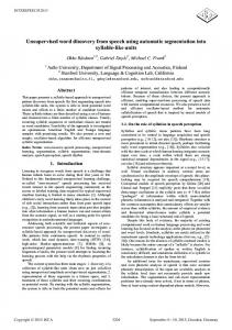
Fig. 2: Top: Spectrogram of the sentence 22a (“two two”) spoken by TiDigits speaker cb. Bottom: block and state labels generated by the model trained on 10 speakers make the block structure, that the method infers from the data, stand out. It is evident that the number of states per block becomes more even as the amount of training data increases. This is also reflected in the use of each block by the model. In the leftmost model, trained on only one speaker, some of the blocks are seldom used, whereas, in the other two models, all blocks are employed to represent particular segments of the speech signal. Table 1 also reports the average length of the pronunciation of each word in terms of blocks and the Levenshtein (edit) distance between different pronunciations within and between words. As can be seen, the within word edit distances are much lower than the between word distances. The latter approach the length of the pronunciations in terms of blocks, indicating that the block representation automatically inferred by the model may be a stable and discriminative rep-

states

blocks

0 10

resentation of words for this data set. Figure 2 shows an example extracted from the database. The top plot depicts the spectrogram of the utterance “22a” spoken by speaker “cb”. The utterance contains, besides some impulsive noise at the beginning, the utterance “two two”. The bottom plot shows the evolution of the state and block labels as predicted by the model. This plot shows that, in spite of the fact that the state labels can vary for the two pronunciations of the word “two”, the sequence of block labels is much more consistent. 5. CONCLUSIONS In this paper we describe the implementation and application to speech of a recently proposed method for inferring the topology of a nearly block diagonal hidden Markov model from the data. We tested the method on a data set containing continuously spoken digits and show that the topology of the resulting model is consistent with linguistic interpretations of the data. In particular, the blocks that emerge form stable and discriminative representations of words in this small vocabulary case. Future work could include testing if this model is suitable for automatic speech recognition. In order to do this, it is necessary to optimise the implementation to make it possible test the method on larger amounts of data. Another interesting possibility is to modify the block probability function to better suit the data found in speech by encouraging a stronger leftto-right pattern within the blocks. Another interesting development would be to perform the inference in a hierarchical way in the attempt to find larger linguistic units from the sub-word units found in this study.

3750

6. REFERENCES [1] M. J. Beal, Z. Ghahramani, and C. E. Rasmussen, “The infinite hidden markov model,” in Advances in neural information processing systems, 2001, pp. 577–584. [2] T. S. Stepleton, Toward versatile structural modification for bayesian nonparametric time series models, Ph.D. thesis, Carnegie Mellon University, 2010. [3] T. S. Stepleton, Z. Ghahramani, G. J. Gordon, and T. S. Lee, “The block diagonal infinite hidden markov model,” in Proc of AI & Statistics, 2009, pp. 552–559. [4] J. Van Gael, Y. Saatci, Y. W. Teh, and Z. Ghahramani, “Beam sampling for the infinite hidden markov model,” in Proc. of ICML. ACM, 2008, pp. 1088–1095. [5] R. Leonard, “A database for speaker-independent digit recognition,” in Proc. IEEE ICASSP, mar 1984, vol. 9, pp. 328 – 331. [6] C-H. Lee, F.K. Soong, and B-H. Juang, “A segment model based approach to speech recognition,” in Proc. of ICASSP, 1988, vol. 1, pp. 501–504. [7] T. Svendsen, K.K. Paliwal, E. Harborg, and P.O. Husoy, “An improved sub-word based speech recognizer,” in Proc. of ICASSP, 1989, vol. 1, pp. 108–111. [8] M. Bacchiani, M. Ostendorf, Y. Sagisaka, and K. Paliwal, “Design of a speech recognition system based on acoustically derived segmental units,” in Proc. of ICASSP, 1996, vol. 1, pp. 443–446. [9] M.A.H. Huijbregts, M. McLaren, and D.A. van Leeuwen, “Unsupervised acoustic sub-word unit detection for query-by-example spoken term detection,” in Proc. Interspeech, 2011. [10] P O’Grady, “Discovering speech phones using convolutive non-negative matrix factorisation with a sparseness constraint,” Neurocomputing, vol. 72, no. 1-3, pp. 88– 101, 2008. [11] O. R¨as¨anen, “A computational model of word segmentation from continuous speech using transitional probabilities of atomic acoustic events,” Cognition, vol. 120, no. 2, pp. 149 – 176, 2011. [12] Alex S. Park and James R. Glass, “Unsupervised pattern discovery in speech,” IEEE Trans. Audio, Speech and Lang. Proc., vol. 16, no. 1, 2008.

[14] V. Stouten, K. Demuynck, and H. van Hamme, “Discovering phone patterns in spoken utterances by nonnegative matrix factorization,” IEEE Signal Processing Lett., vol. 15, pp. 131–134, 2008. [15] J. Driesen, L. ten Bosch, and H. van Hamme, “Adaptive non-negative matrix factorization in a computational model of language acquisition,” in Proc. Interspeech, 2009. [16] C. Yu, L. B. Smith, and A. F. Pereira, “Grounding word learning in multimodal sensorimotor interaction,” in Proc. Annual Conf. Cog. Science Soc., 2008, pp. 1017– 1022. [17] G. Salvi, L. Montesano, A. Bernardino, and J. SantosVictor, “Language bootstrapping: Learning word meanings from perception-action association,” IEEE Trans. Syst., Man, and Cybern., Part B: Cybern., 2011. [18] G. E. Hentera and B. W. Kleijn, “Picking up the pieces: Causal states in noisy data, and how to recover them,” Patt. Rec. Letters, vol. 34, no. 5, pp. 587–594, 2013. [19] C. R. Shalizi and K. L. Shalizi, “Blind construction of optimal nonlinear recursive predictors for discrete sequences,” in Proc. of UAI, 2004, pp. 504–511. [20] N. Vanhainen and G. Salvi, “Word discovery with beta process factor analysis,” in Proc. of Interspeech, Portland, OR, USA, Sept. 2012. [21] J. Paisley and L. Carin, “Nonparametric factor analysis with beta process priors,” in Proc. Annual Int. Conf. on Machine Learning, 2009, pp. 777–784. [22] L. Qin and A. Rudnicky, “Oov word detection using hybrid models with mixed types of fragments,” in Proc. of Interspeech, 2012, pp. 2450–2453. [23] T. Mertens and S. Seneff, “Subword-based automatic lexicon learning for speech recognition,” in Proc of ASRU, 2011, pp. 243–248. [24] Y. W. Teh, M. I. Jordan, M. J. Beal, and D. M. Blei, “Hierarchical Dirichlet processes,” Journal of the American Statistical Association, vol. 101, no. 476, pp. 1566– 1581, 2006. [25] “The hidden Markov http://htk.eng.cam.ac.uk.

[13] G. Aimetti, R. K. Moore, and L. ten Bosch, “Discovering an optimal set of minimally contrasting acoustic speech units: A point of focus for whole-word pattern matching,” in Proc. Interspeech, 2010, pp. 310 – 313.

3751

model

toolkit

(HTK),”