pattern recognition using composite features - CiteSeerX

Ph.D. DISSERTATION

PATTERN RECOGNITION USING COMPOSITE FEATURES

"! $#&%$* '( ),.+( -01 / BY CHUNGHOON KIM

AUGUST 2007

DEPARTMENT OF ELECTRICAL ENGINEERING AND COMPUTER SCIENCE COLLEGE OF ENGINEERING SEOUL NATIONAL UNIVERSITY

PATTERN RECOGNITION USING COMPOSITE FEATURES

"! $#&%$* '( ),.+( -01 / =< ? > A B@ NQZP [ Y E CFHI GFA]7 \ _a ^ `cbef d N g P lnm 2007 hj( i 6 k oqp.f r s$t NQ P 8 6 s$t NQvP wyu x zq(}{ | ~c} " q LJ MONQP / q

2 4 57 3 8: 6 ;9 DE CFHI GF K LJ MONQSP RUWT V0X

D/ q Z L J MONSQ P RUWT V0X NQZP [ Y E CFHI GF ),+( N g P lnm 2007 hj( i 7 k [ Y wyu x : =< +( j [ Y wyu xD : =< ? > B @ [Y wyu x : U T [Y wyu x : ¢¡¤¦ £ ;¥ [Y wyu x : ¨ § ©«5 ª

Abstract Pattern recognition aims to classify a pattern into one of the predefined classes. A pattern is represented by a set of variables, which are called primitive variables in this dissertation. For a better classification performance, feature extraction has been widely used to obtain new features from primitive variables. This reduces the number of variables while preserving as much discriminative information as possible. In this dissertation, the main focus is on the feature extraction for pattern recognition. A new method of extracting composite features is derived and then applied to several problems such as eye detection, face recognition, and ordinary pattern classification problems. The method of extracting composite features is first derived from face images. In appearance-based models for face recognition, the intensity of each pixel in a face image is used as a primitive variable. In the proposed method, a composite vector is composed of a number of pixels inside a window on an image. The covariance of composite vectors is obtained from the inner product of composite vectors and can be considered as a generalized form of the covariance of pixels. It contains information on statistical dependency among multiple pixels. The size of the covariance matrix can be controlled by changing the window size or by overlapping the windows. This is a great advantage because manipulation of a large-sized covariance matrix can be avoided and consequently the small sample size problem can be solved. The proposed C-LDA is a linear discriminant analysis (LDA) using the covariance of composite vectors. In C-LDA, features are obtained by linear combinations of the composite vectors. These extracted features are called composite features because each feature is a vector whose dimension is equal to the dimension of the composite vector. This composite feature is further reduced by using a downscaling technique because there

are usually strong correlations among the elements of the composite feature. An image can be represented by these reduced composite features, each of which is a small-sized vector. In the case of C-LDA, the small sample size problem rarely occurs and the number of extracted features can be larger than the number of classes because the within-class and between-class scatter matrices have full ranks. The C-LDA is applied to several classification problems. First, composite features are used to detect eyes for face recognition in a facial image. In eye detection, positive samples for eyes are similar and they can be assumed to be normally distributed, while negative samples are not. In this case, it is better to use the objective function in biased discriminant analysis (BDA), rather than the function in LDA. The proposed C-BDA is a biased discriminant analysis using the covariance of composite vectors, which is a variant of C-LDA. In the hybrid cascade detector constructed for eye detection, Haar-like features are used in the earlier stages and composite features obtained from C-BDA are used in the later stages. The experimental results for the FERET database show that the hybrid cascade detector provides eye detection rates of 99.0% and 96.2% for 200 validation images and 1000 test images, respectively. Second, composite features are used for face recognition, where the features are obtained from C-LDA. Comparative experiments are performed using the FERET, CMU, and ORL databases of facial images. The experimental results show that the proposed C-LDA provides the best recognition rate among several methods in all of the tests and provides the robust performance to the variations in facial expression, illumination, and eye coordinates. Third, three types of C-LDA are derived for classification problems of ordinary data sets, which are not image data sets. The proposed C-LDA(E), C-LDA(C), and C-LDA(N) can be considered as generalizations of LDA using the Euclidean distance, LDA using

the Chernoff distance, and the nonparametric discriminant analysis, respectively. Experimental results on several data sets indicate that C-LDA provides better classification results than the other methods. Especially on the Sonar data set, C-LDA(E) with the Parzen classifier shows much better performance, compared to previously reported results. In summary, C-LDA is a general method to use the covariance of composite vectors instead of the covariance of primitive variables, and can be applied to several classification problems. C-LDA shows a much better performance than the other methods, especially when adjacent primitive variables are strongly correlated as in image data sets and the Sonar data set.

Keywords: pattern recognition, feature extraction, composite feature, face recognition, eye detection, classification, covariance matrix, linear discriminant analysis, biased discriminant analysis, nonparametric discriminant analysis

Student Number: 2002-23516

Contents 1

2

3

Introduction

1

1.1

Previous works for feature extraction . . . . . . . . . . . . . . . . . . . .

1

1.2

Motivation . . . . . . . . . . . . . . . . . . . . . . . . . . . . . . . . . .

4

1.3

Organization of the Dissertation . . . . . . . . . . . . . . . . . . . . . .

5

Linear Discriminant Analysis Using the Covariance of Composite Vectors (C-LDA)

7

2.1

Composite vectors and their covariance in images . . . . . . . . . . . . .

8

2.2

Derivation of C-LDA . . . . . . . . . . . . . . . . . . . . . . . . . . . . 10

2.3

Interpretation of C-LDA . . . . . . . . . . . . . . . . . . . . . . . . . . 15

2.4

Distance metrics and confidence measure in the classification . . . . . . . 20

2.5

Bayes error in C-LDA . . . . . . . . . . . . . . . . . . . . . . . . . . . . 21

Eye Detection Using Haar-like Features and Composite Features 3.1

25

Hybrid cascade detector using Haar-like features and composite features . 26 3.1.1

Haar-like features obtained from Adaboost . . . . . . . . . . . . 27

3.1.2

Composite features obtained from the biased discriminant analysis 29

3.1.3

Hybrid cascade detector for eye detection . . . . . . . . . . . . . 34 i

3.2

4

5

6

Experimental results for eye detection . . . . . . . . . . . . . . . . . . . 35 3.2.1

Training results . . . . . . . . . . . . . . . . . . . . . . . . . . . 35

3.2.2

Test results . . . . . . . . . . . . . . . . . . . . . . . . . . . . . 40

Face Recognition Using Composite Features

45

4.1

Experimental results for the Color FERET database . . . . . . . . . . . . 46

4.2

Experimental results for the CMU PIE database . . . . . . . . . . . . . . 55

4.3

Experimental results for the ORL database . . . . . . . . . . . . . . . . . 58

Pattern Classification Using Composite Features

61

5.1

C-LDA(E) for pattern classification

5.2

Variants of C-LDA(E) . . . . . . . . . . . . . . . . . . . . . . . . . . . . 66

5.3

Experimental results for classification problems . . . . . . . . . . . . . . 68

Conclusions

. . . . . . . . . . . . . . . . . . . . 62

79

ii

List of Figures 2.1

Several types of windows, each of which makes a composite vector . . . .

2.2

Schematic diagram of C-LDA . . . . . . . . . . . . . . . . . . . . . . . 12

2.3

The ratio of the first b largest eigenvalues to the total sum of eigenvalues of the covariance matrix

8

. . . . . . . . . . . . . . . . . . . . . . . . . . 14

2.4

Images used in C-LDA . . . . . . . . . . . . . . . . . . . . . . . . . . . 16

2.5

Projection process to obtain composite features in C-LDA . . . . . . . . 19

2.6

Projection process to obtain reduced composite features directly, in C-LDA 19

2.7

Bayes errors in the subspaces obtained by C-LDA . . . . . . . . . . . . . 22

3.1

Seven prototypes of the Haar-like features . . . . . . . . . . . . . . . . . 28

3.2

Eye and noneye samples used in Adaboost learning . . . . . . . . . . . . 29

3.3

Ten features selected by Adaboost . . . . . . . . . . . . . . . . . . . . . 29

3.4

Classification rates on the validation set . . . . . . . . . . . . . . . . . . 30

3.5

Eye and noneye samples used in C-BDA . . . . . . . . . . . . . . . . . . 32

3.6

Ten projection vectors obtained by C-BDA . . . . . . . . . . . . . . . . . 33

3.7

ROC curves comparing C-BDA with BDA . . . . . . . . . . . . . . . . . 33

3.8

Schematic diagram of the hybrid cascade detector . . . . . . . . . . . . . 35

3.9

Five sizes of detection windows for eye detection . . . . . . . . . . . . . 36 iii

3.10 Detection results on a validation image . . . . . . . . . . . . . . . . . . . 38 3.11 Composite features vs. Haar-like features . . . . . . . . . . . . . . . . . 39 3.12 Detection results on a validation image . . . . . . . . . . . . . . . . . . . 40 3.13 Eye detection results on 200 validation images . . . . . . . . . . . . . . . 41 3.14 Eye detection results on 1000 test images . . . . . . . . . . . . . . . . . 42 3.15 Examples of the correct detection . . . . . . . . . . . . . . . . . . . . . . 43 3.16 Examples of the incorrect detection

. . . . . . . . . . . . . . . . . . . . 44

4.1

Sample images cropped to the size of 120×100 . . . . . . . . . . . . . . 46

4.2

Recognition rates of C-LDA using different windows . . . . . . . . . . . 47

4.3

Recognition rates of C-LDA with respect to the overlapping and the downscaling factor . . . . . . . . . . . . . . . . . . . . . . . . . . . . . 49

4.4

Recognition rates of C-LDA using four different distance metrics . . . . . 50

4.5

Probability distributions of the confidence measure . . . . . . . . . . . . 51

4.6

Comparative experiments of the four feature extraction methods . . . . . 52

4.7

Recognition rates of C-LDA with manually and automatically located eye coordinates . . . . . . . . . . . . . . . . . . . . . . . . . . . . . . . 53

4.8

Sample images of the CMU database . . . . . . . . . . . . . . . . . . . . 56

4.9

Recognition rates of the four feature extraction methods for the CMU database . . . . . . . . . . . . . . . . . . . . . . . . . . . . . . . . . . . 57

4.10 Sample images of the ORL database . . . . . . . . . . . . . . . . . . . . 58 4.11 Recognition rates of the four feature extraction methods for the ORL database . . . . . . . . . . . . . . . . . . . . . . . . . . . . . . . . . . . 59 5.1

Composite vectors in a pattern represented as a vector, motivated from images . . . . . . . . . . . . . . . . . . . . . . . . . . . . . . . . . . . . 62 iv

5.2

Classification process by C-LDA(E) . . . . . . . . . . . . . . . . . . . . 65

5.3

Classification rates of C-LDA(E) for various values of l and m . . . . . . 70

5.4

Classification rates of C-LDA(E) for various orderings of primitive variables . . . . . . . . . . . . . . . . . . . . . . . . . . . . . . . . . . . . . 74

5.5

Classification rates of C-LDA(E) for various overlapping intervals . . . . 75

5.6

The average values of 60 primitive variables in each class of the Sonar data set, represented in gray scales . . . . . . . . . . . . . . . . . . . . . 76

v

vi

List of Tables 4.1

C-LDA vs. LDA . . . . . . . . . . . . . . . . . . . . . . . . . . . . . . 54

5.1

Data sets used in the experiments . . . . . . . . . . . . . . . . . . . . . . 68

5.2

Classification rates and optimal parameters

vii

. . . . . . . . . . . . . . . . 71

viii

Chapter 1

Introduction Pattern recognition aims to classify a pattern into one of the predefined classes. A pattern is represented by a set of variables, which are called primitive variables in this dissertation. For a better classification performance, feature extraction has been widely used to obtain new features from primitive variables [1–3]. This reduces the number of variables while preserving as much discriminative information as possible. In this dissertation, the main focus is on the feature extraction for pattern recognition. A new method of extracting composite features is derived and then applied to several problems such as eye detection, face recognition, and ordinary pattern classification problems.

1.1 Previous works for feature extraction Feature extraction is a process of finding features which are effective for discriminating patterns, in which features are usually obtained by linear combinations of the primitive variables. There are several reasons for performing feature extraction in pattern recognition [2]: 1

Chapter 1. Introduction 1) to reduce the number of variables, resulting in reduced computation time for classification and reduced memory requirements for storage; 2) to reduce redundancy in a pattern; 3) to provide a relevant set of features for a classifier, resulting in improved performance, particularly from simple classifiers. The principal component analysis (PCA) is a well-known method for feature extraction. PCA originated from the work by Pearson [4], and it aims to find a linear transform that maximizes the scatter of projected patterns. The eigenvectors corresponding to the largest eigenvalues of the covariance matrix are used for the projection vectors, in PCA [5]. Since PCA does not use class information, it is an unsupervised method for feature extraction. It tries to find only the most expressive features in terms of mean-square error [3]. Meanwhile, the linear discriminant analysis (LDA) uses the class information associated with each pattern for obtaining the most discriminant features. The objective of LDA is to find a linear transform that maximizes the ratio of the between-class scatter and the within-class scatter [1]. It is very effective for classifying patterns if the within-class variance is small while the between-class variance is large. However, there are two limitations in applying LDA. If the number of primitive variables is larger than the number of training samples, the within-class scatter matrix becomes singular and LDA cannot be applied directly. This problem is called the small sample size (SSS) problem [1]. The other limitation is that the number of features that can be extracted is at most one less than the number of classes. This becomes a serious problem in binary classification problems, in which only a single feature can be extracted by LDA. These two limitations are attributed to the rank deficiencies of the within-class 2

Chapter 1. Introduction scatter matrix (SW ) and the between-class scatter matrix (S B ). In order to solve the SSS problem, several approaches such as the PCA preprocessing [6,7], null-space method [8,9], and direct LDA [10,11] have been introduced. Belhumeur et al. proposed the Fisherface method for face recognition, in which PCA is applied first in order to make SW nonsingular and then LDA is applied to find the projection vectors called Fisherfaces [6]. The Null-space LDA (N-LDA) [8, 9] is a new approach to solve the SSS problem. The key idea of this method is that the null space of S W contains useful discriminative information [8, 12]. By projecting samples into the null space of SW using W1 that satisfies W1T SW W1 = 0, all the samples in each class are projected to one point. Then, a set of eigenvectors W 2 of SB is found in the null space of SW , where the columns of W2 are the eigenvectors corresponding to larger eigenvalues. The N-LDA method uses the projection W T = W2T W1T . There are also several approaches that can increase the number of extracted features by modifying the between-class scatter matrix in LDA. Fukunaga and Mantock proposed the nonparametric discriminant analysis (NDA) which uses the nonparametric between-class scatter matrix [1, 13]. Brunzell and Eriksson proposed the Mahalanobis distance-based method [14]. Recently, Loog and Duin [15] used the Chernoff distance [16] between two classes to generalize the between-class scatter matrix. The Bayesian method is another approach for feature extraction, which is based on a probabilistic model [17, 18]. This method uses a similarity measure obtained from the Bayes’ theorem, where intrapersonal and extrapersonal variations are modeled as Gaussian distributions in each principal subspace. This approach is called the dual eigenspace method because two PCA projections are required [18]. A unified subspace method [7] that uses PCA, Bayesian and then LDA sequentially was recently introduced for face recognition. This method is based on the Fisherface framework, and uses the maximum 3

Chapter 1. Introduction likelihood technique after applying PCA, which projects samples into the intrapersonal eigenspace. This technique is similar to the whitening process in LDA except for the dimensionality reduction.

1.2 Motivation All of the methods described in the above use the covariance of primitive variables. On the other hand, Yang et al. proposed a straightforward image projection technique called the two-dimensional principal component analysis (2DPCA) for face recognition [19, 20]. An image is represented as a matrix and its transpose is multiplied by itself to obtain a covariance matrix. Since each element of the covariance matrix is obtained from the covariance of column vectors in the image matrix, the size of the covariance matrix is determined by the number of columns in the image matrix. Recently, Yang et al. [21] and Xiong et al. [22] introduced 2DLDA, which is a linear discriminant analysis using the covariance of column vectors in the image matrix. For non-image classification problems, Chen et al. introduced MatFLDA, where a pattern is represented as a matrix and a covariance matrix is obtained from the covariance of row vectors in the matrix [23]. Although the SSS problem rarely occurs in 2DLDA, its performance on face recognition was not impressive [21, 22, 24]. As pointed out in [25] and [26], 2DLDA is similar to LDA using each row of an image as an individual sample. This means there are f r samples per image, where fr is the number of rows in the image. Therefore, the number of samples in 2DLDA is fr times larger than that in ordinary LDA. This makes 2DLDA avoid the SSS problem. However, it is inappropriate to use all of the rows of an image as samples belonging to the same class. In this dissertation, a new method of extracting composite features is proposed. It 4

Chapter 1. Introduction is first derived from face images. In appearance-based models for face recognition, the intensity of each pixel in a face image is usually used as a primitive variable. In the proposed method, a composite vector is composed of a number of pixels inside a window on an image. The covariance of composite vectors is obtained from the inner product of composite vectors and can be considered as a generalized form of the covariance of pixels. It contains information on statistical dependency among multiple pixels. The size of the covariance matrix can be controlled by changing the window size or by overlapping the windows. This is a great advantage because manipulation of a large-sized covariance matrix can be avoided and consequently the SSS problem can be solved. The proposed C-LDA is a linear discriminant analysis using the covariance of composite vectors [27–29]. In C-LDA, features are obtained by linear combinations of the composite vectors. These extracted features are called composite features because each feature is a vector whose dimension is equal to the dimension of the composite vector. This composite feature is further reduced by using a downscaling technique because there are usually strong correlations among the elements of the composite feature. An image can be represented by these reduced composite features, each of which is a small-sized vector. In the case of C-LDA, the SSS problem rarely occurs and the number of extracted features can be larger than the number of classes because the within-class and between-class scatter matrices have full ranks.

1.3 Organization of the Dissertation This dissertation is organized as follows. In Chapter 2, we define the composite vector in images and derive C-LDA using the covariance of composite vectors. We also investigate the characteristics of C-LDA. In Chapter 3, we derive C-BDA for eye detection, which is 5

Chapter 1. Introduction a biased discriminant analysis (BDA) using the covariance of composite vectors. We also construct a hybrid cascade detector, where Haar-like features and composite features are used in earlier stages and later stages, respectively. Experimental results for eye detection are presented at the end of the chapter. In Chapter 4, we use the composite features for face recognition, where the features are obtained from C-LDA. Experimental results for the FERET [30], CMU [31], and ORL [32] databases of facial images are presented. In Chapter 5, three types of C-LDA, i.e., C-LDA(E), C-LDA(C), and C-LDA(N), are derived for classification problems of ordinary data sets, which are not image data sets. They are generalizations of LDA using the Euclidean distance, LDA using the Chernoff distance, and NDA, respectively. Experimental results on several data sets are presented at the end of the chapter. Finally, conclusions follow in Chapter 6.

6

Chapter 2

Linear Discriminant Analysis Using the Covariance of Composite Vectors (C-LDA)

In this chapter, we first define a composite vector which consists of a number of pixels inside a window on an image. Then, we propose C-LDA which is a linear discriminant analysis using the covariance of composite vectors [27–29]. In C-LDA, features are obtained by linear combinations of the composite vectors. Those extracted features are called composite features because each feature is a vector whose dimension is equal to the dimension of the composite vector. Unlike [29], we differentiate the composite feature from the composite vector in order to avoid confusion in terminology. 7

Chapter 2. Linear Discriminant Analysis Using the Covariance of Composite Vectors (C-LDA) (a)

(b) (c) (d) (e)

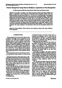
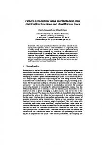
Figure 2.1: Several types of windows, each of which makes a composite vector: The window sizes of (a), (b), (c), (d), and (e) are 120×1, 1×100, 6×5, 12×10, and 24×20, respectively.

2.1 Composite vectors and their covariance in images In face recognition, patterns are composed of two-dimensional face images. There are more than tens of thousands of pixels in a face image, and each pixel is strongly correlated with its neighboring pixels. Therefore, the covariance matrix obtained from pixelwise covariances is very large and contains a lot of redundant information. Let us consider a composite vector composed of a number of pixels inside a window on an image. Let F ∈ Rfr ×fc denote a face image, where fr and fc are the height and width of the image. Let H denote a set of windows {H 1 , H2 , . . . , Hn } in the image. Each window Hi ∈ Rhr ×hc has l (= hr × hc ) pixels, where hr and hc are the height and width of the window. Then, the number of windows, n is

p l

where p is the total number of pixels in F .

Obviously, more windows can be obtained if neighboring windows overlap each other. Figure 2.1 shows several types of windows. In the figure, the size of the face image is 120×100 (pixels), and the window sizes of (a), (b), (c), (d), and (e) are 120×1, 1×100, 6×5, 12×10, and 24×20, respectively. 8

Chapter 2. Linear Discriminant Analysis Using the Covariance of Composite Vectors (C-LDA) Let the set of composite vectors X be {x 1 , x2 , . . . , xn }, where x1 = OL (H1 ), x2 = OL (H2 ), and so on. Here, OL (·) is the lexicographic ordering operator that transforms a matrix into a vector by ordering the rows of the matrix one after the other [38]. Therefore, xi becomes a l-dimensional vector. Let C denote a covariance matrix based on the composite vectors. The element cij of C is defined as ¯ i )T (xj − x ¯ j )], cij = E[(xi − x

i, j = 1, 2, . . . , n,

(2.1)

¯ i and x ¯ j are the mean vectors of xi and xj , respectively. Note that cij corresponds where x to the total sum of covariances between the corresponding pixels in H i and Hj . It contains information on statistical dependency among multiple pixels. Then, the covariance matrix C is computed as [2] C=

N 1 X (X(k) − M )(X(k) − M )T , N

(2.2)

k=1

¯ n ]T , and N is x1 . . . x where X(k) = [x1 (k) . . . xn (k)]T for the kth sample, M = [¯ the total number of samples. Note that X(k) ∈ R n×l and C ∈ Rn×n . Let us consider the rank of C. Let χj (k), mj ∈ Rn denote the column vectors of X(k) and M , respectively. Then X(k) = [χ 1 (k) . . . χl (k)] and M = [m1 . . . ml ]. We rewrite (2.2) as N l 1 XX C= (χj (k) − mj )(χj (k) − mj )T . N

(2.3)

k=1 j=1

There are at most N l linearly independent vectors in (2.3), and consequently the rank of C is at most N l. Also, (χj (k) − mj )’s are not linearly independent because they are P related by N k=1 (χj (k) − mj ) = 0 for j = 1, . . . , l. Therefore, the rank of C is rank(C) ≤ min(n, (N − 1)l), 9

(2.4)

Chapter 2. Linear Discriminant Analysis Using the Covariance of Composite Vectors (C-LDA) q and is usually n if n = pl and l ≥ Np−1 . When using pixelwise covariances (l = 1), the rank of the covariance matrix is smaller than or equal to min(p, (N − 1)), and is usually (N − 1), which causes the small sample size (SSS) problem [1]. However, when using the covariance of composite vectors, the size of C can be reduced greatly so that the rank of C is equal to the number of composite vectors. This enables us to avoid manipulation of the large-sized covariance matrix and to solve the SSS problem.

2.2 Derivation of C-LDA The composite vectors and their covariance are obtained in the previous section. C-LDA is a linear discriminant analysis using the covariance of composite vectors, instead of the pixelwise covariance. Before deriving C-LDA, let us define a within-class scatter matrix CW and a between-class scatter matrix C B . Assume that each training sample belongs to one of D classes, c1 , c2 , . . . , cD , and that there are Ni samples for class ci . As in the covariance matrix C, CW ∈ Rn×n is defined as CW =

D X

pi {

i=1

1 X (X(k) − Mi )(X(k) − Mi )T }, Ni

(2.5)

k∈Ii

where Mi =

1 X X(k). Ni k∈Ii

Here pi is a prior probability that a sample belongs to class c i , and Ii is the set of indices of the training samples belonging to class c i . CB ∈ Rn×n is also defined as CB =

D X

pi (Mi − M )(Mi − M )T .

(2.6)

i=1

As in (2.4), the rank of CW is rank(CW ) ≤ min(n, (N − D)l). 10

(2.7)

Chapter 2. Linear Discriminant Analysis Using the Covariance of Composite Vectors (C-LDA) q p If l ≥ N −D and n = pl , then (N −D)l ≥ n and CW has full rank in most cases. When using pixelwise covariances, the rank is smaller than or equal to min(p, (N − D)), and is usually N − D, which causes the SSS problem. However, this problem will not occur in C-LDA, and consequently PCA preprocessing is not necessary. And the rank of C B is rank(CB ) ≤ min(n, (D − 1)l).

(2.8)

In LDA (l = 1), the rank is smaller than or equal to min(p, (D − 1)), which is the maximum number of features that can be extracted. However, one can extract features up to rank(CB ), which is larger than D − 1, in C-LDA. It is important to emphasize that the problems caused by rank deficiencies of C W and CB can be avoided by using composite vectors. In C-LDA, the set of projection vectors W L , which maximizes the ratio of the betweenclass scatter and the within-class scatter, is obtained by WL = arg max W

|W T CB W | , |W T CW W |

(2.9)

where WL = [w1 . . . wm ] ∈ Rn×m . This can be computed in two steps as in LDA [2]. 1

First, CW is transformed to an identity matrix by (ΨΘ − 2 ) ∈ Rn×n , where Ψ and Θ are 0 and C 0 the eigenvector and diagonal eigenvalue matrices of C W , respectively. Let CW B

denote the within-class and between-class scatter matrices after whitening, respectively. 1

1

0 0 = (ΨΘ− 2 )T C (ΨΘ− 2 ). Second, C 0 is diagonalized by = I and CB Then CW B B

Φ ∈ Rn×m , where the columns vectors of Φ are the m eigenvectors corresponding to 0 . Therefore, W is expressed with m projection vectors the m largest eigenvalues of CB L 1

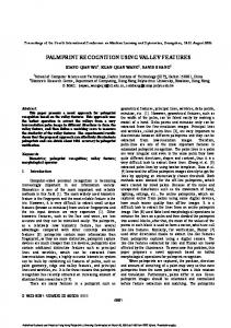
of ΨΘ− 2 Φ. The four projection vectors from w 1 to w4 are represented as matrices in Fig. 2.2. These correspond to the Fisherfaces [6], but the dimension of each projection vector is n, not p. In this case, n is 361 (19×19) because the windows of 12×10 pixels 11

Chapter 2. Linear Discriminant Analysis Using the Covariance of Composite Vectors (C-LDA) C-LDA

(a)

Training image

(b)

Projection vectors

(c)

Composite features

Reduced composite features

Figure 2.2: Schematic diagram of C-LDA: (a) The projection vectors are obtained from C-LDA using the covariance of composite vectors. (b) The composite features are obtained by projecting the composite vectors. Note that the composite features have the same size as the composite vectors. (c) The composite features are further reduced by applying a downscaling operator. In this case, the downscaling factor r is 30. are used and they overlap either horizontally or vertically by 50%. In the training image of Fig. 2.2, there are nine small rectangles on the face. The size of the face image is 120×100 (pixels), and each small rectangle contains 6×5 pixels. Here, a composite vector consists of 120 pixels inside a 12×10 rectangular window, i.e., l = 120, and four adjacent windows overlap either horizontally or vertically by 50%. Then, the set of composite features Y (k) is obtained from X(k) as Y (k) = WL T X(k),

k = 1, 2, . . . , N,

where Y (k) ∈ Rm×l has m composite features [y1 (k) y2 (k) . . . ym (k)]T , and each composite feature yi (k) is a l-dimensional vector. It is noted that C-LDA with l = 1 is 12

Chapter 2. Linear Discriminant Analysis Using the Covariance of Composite Vectors (C-LDA) the same as LDA. The first four features from O L −1 (y1 (k)) to OL −1 (y4 (k)) are shown in Fig. 2.2, where OL −1 (·) is the inverse of the lexicographic ordering operator. Note that the size of yi (k) is 120, which is the same as that of the composite vector. It is burdensome to use yi (k) directly because it has a large number of elements. However, the dimension of yi (k) can be further reduced if the elements of y i (k) are strongly correlated with each other. Let us consider N samples of the ith composite feature {y i (1), yi (2), . . . , yi (N )}. The covariance matrix can be obtained from these samples, and its size is l×l. The eigenvalues of this covariance matrix reveal how much the elements of y i (k) are correlated. When the ratio of the first b largest eigenvalues to the total sum of eigenvalues is close to 1, yi (k) can be well represented by the b eigenvectors corresponding to the b largest eigenvalues. In this case, it may be redundant to use all of the elements of y i (k). Figure 2.3 shows the ratio of the first b largest eigenvalues to the total sum of eigenvalues of the covariance matrix obtained from the 400 training images in the Color FERET database. For more details about the training images, see Section 4.1. When i = 1, the ratios are 97.8%, 99.0%, and 99.7% for b=1, 2, and 4, respectively. This means that most samples of y1 (k) (k = 1, . . . , N ) are concentrated on a few principal axes, which implies that the correlations among the elements of y 1 (k) are very strong. Therefore the dimension of the composite feature y1 (k) can be reduced significantly without losing much information. In order to reduce the dimension of y i (k), we may use PCA, but we use a simple downscaling technique instead. The ratios in Fig. 2.3 decrease as i increases, which implies that the reduced dimension of y i (k) should be larger as i increases. However, we apply the same downscaling factor r for y i (k) regardless of i because the first few composite features have most of the discriminative information. Then Y (k) becomes l

Z(k) = [z1 (k) z2 (k) . . . zm (k)]T , where zi (k) = OL [OD(r) {OL −1 (yi (k))}] ∈ R r , 13

Chapter 2. Linear Discriminant Analysis Using the Covariance of Composite Vectors (C-LDA)

PSfrag replacements

Ratio of the first b largest eigenvalues (%)

100

b=1 b=2 b=4

80

60

40

20

0

0

50

100

ith composite feature

Figure 2.3: The ratio of the first b largest eigenvalues to the total sum of eigenvalues of the covariance matrix, which is obtained from the ith composite feature y i (k) of N samples.

14

Chapter 2. Linear Discriminant Analysis Using the Covariance of Composite Vectors (C-LDA) (i = 1, . . . , m). Here OD(r) is a downscaling operator with factor r, where r elements are represented by their average value. As a result of O D(r) (·), the number of elements in OL −1 (yi (k)) are reduced from l to rl . The four reduced features from z1 (k) to z4 (k) are represented as matrices in Fig. 2.2. In this case, r is set to 30, so the 6×5 elements of each composite feature are represented by their average value. Note that Z(k) corresponds to the set of reduced composite features from the kth image, by C-LDA.

2.3 Interpretation of C-LDA C-LDA is derived from the linear discriminant analysis using the covariance of composite vectors in the previous section. We interpret C-LDA from another point of view, not from the view of the composite vectors. As in (2.3), C W can be represented using the column vectors of X(k). Let mij ∈ Rn (j = 1, . . . , l) denote the column vectors of M i . Then we rewrite (2.5) as CW =

D X i=1

pi [

l 1 X X { (χj (k) − mij )(χj (k) − mij )T }]. Ni

(2.10)

k∈Ii j=1

The number of outer products of vectors in (2.10) is N l, which is l times larger than that in LDA. It is because X(k) has l column vectors of χ j (k). Figure 2.4(a) shows l images of χj (k) for some k. In this case, l and n are 120 and 361, respectively, because the windows of 12×10 pixels are used and they overlap either horizontally or vertically by 50%. In this figure, each image corresponds to O L −1 (χj (k)) for j = 1, . . . , 120. Let the (i, j) image denote the image in the ith row and jth column of the figure, and the (i, j) pixel in an image denote the pixel in the ith row and jth column of the image. From the viewpoint of composite vectors, the (1,1) image in the top left corner consists of n pixels obtained from the first element of each composite vector, and the (1,2) image consists of n pixels obtained from the second element of each composite vector. For example, 15


(a) Training images corresponding to χj (k)

(b) Difference images corresponding to (χj (k) − mij )

Figure 2.4: Images used in C-LDA. 16

Chapter 2. Linear Discriminant Analysis Using the Covariance of Composite Vectors (C-LDA) the (1,1) pixel in the (1,1) image corresponds to the (1,1) pixel in the original image F , while the (1,1) pixel in the (1,2) image corresponds to the (1,2) pixel in F . Hence, the (i, j) pixel in the (1,10) image is obtained from the pixel located at nine pixels to the right in F , compared to the (i, j) pixel in the (1,1) image. Likewise, the (i, j) pixel in the (12,1) image is obtained from the pixel located at eleven pixels below in F , compared to the (i, j) pixel in the (1,1) image. As can be seen in the figure, there is no hair on the right side of the (1,1) image, while there are hairs on the right side of the (1,10) image. Also, there is no beard on the bottom side of the (1,1) image, while there is a beard on the bottom side of the (12,1) image. All these 120 images are used for making C W . Therefore, we can expect that C-LDA will provide a robust performance to the variation caused by alignment of faces. From this point of view, C-LDA is similar to LDA using l times more images of smaller size. However, there is a difference between C-LDA and LDA. In C-LDA, (χ j (k)−mij )’s are used for making CW as seen in (2.10). Figure 2.4(b) shows 120 difference images P corresponding to χj (k) − mij for j = 1, . . . , 120. Since mij = N1i k∈Ii χj (k), mij varies depending on j. Meanwhile, the mean image of class c i depends only on i in LDA. Let mi denote the mean image of χj (k) belonging to the class ci , i.e., mi = Pl 1 P i i k∈Ii j=1 χj (k). In LDA, m will be used for making CW , instead of mj . Ni Let us further investigate the relationship between C-LDA and LDA. We rewrite (2.10) as CW =

l X D X 1 X [ pi { (χj (k) − mij )(χj (k) − mij )T }] Ni j=1 i=1

=

l X

k∈Ii

(2.11)

(SW )j ,

j=1

where (SW )j =

PD

1 i=1 pi { Ni

P

k∈Ii (χj (k)

17

− mij )(χj (k) − mij )T } is a within-class

Chapter 2. Linear Discriminant Analysis Using the Covariance of Composite Vectors (C-LDA) scatter matrix obtained from χj (k)’s. Note that χj (k) is an n dimensional vector and n was set to 361 in Fig. 2.4(a). Here, (S W )j corresponds to the within-class scatter matrix obtained from primitive variables in LDA. Since C W in C-LDA can be represented as the sum of l (SW )j ’s, it is a composite of within-class scatter matrices in LDA. This is due to the definition of the covariance of composite vectors in (2.1), where the covariance c ij is defined as the sum of l covariances between the corresponding pixels in x i and xj . Likewise, CB in (2.6) can be represented as CB =

l X D X [ pi (mij − mj )(mij − mj )T ] j=1 i=1

=

l X

(2.12)

(SB )j ,

j=1

where (SB )j =

PD

i i=1 pi (mj

− mj )(mij − mj )T is a between-class scatter matrix ob-

tained from mij ’s. Also, CB in C-LDA is a composite of between-class scatter matrices in LDA. Figure 2.5 shows the schematic diagram of the projection process to obtain composite features in C-LDA. The composite feature in the figure is obtained by projecting the training images. For example, the (1,1) element of the composite feature is obtained by projecting the (1,1) image onto the projection vector, and the (1,2) element is obtained by projecting the (1,2) image. Since the differences between adjacent training images are very small, the correlations between adjacent elements of the composite feature are very strong. This coincides with the analysis on the eigenvalues in Section 2.2. Therefore, the dimension of the composite feature can be reduced significantly. In this case, the downscaling factor r is set to 30, so the 6×5 elements of each composite feature are represented by their average value. If r is chosen, the reduced composite features can be obtained directly without project18


C-LDA

Training images

Projection vector

Composite feature

Reduced composite feature

Figure 2.5: Projection process to obtain composite features in C-LDA.

C-LDA

Downscaled images

Projection vector

Reduced composite feature

Figure 2.6: Projection process to obtain reduced composite features directly, in C-LDA.

19

Chapter 2. Linear Discriminant Analysis Using the Covariance of Composite Vectors (C-LDA) ing all the l training images onto the projection vector. For example, the (1,1) element of the reduced composite feature is the same as the value obtained by projecting the mean of 30 (i, j) images, {(i, j), i=1,. . .,6; j=1,. . .,5}, onto the projection vector. Figure 2.6 shows the schematic diagram of the projection process to obtain reduced composite features directly. In this case, the reduced composite features are obtained by projecting only four images onto the projection vector. Therefore, the computation time to obtain composite features can be reduced significantly.

2.4 Distance metrics and confidence measure in the classification The composite features are obtained from C-LDA using the covariance of composite vectors in Section 2.2. The set of reduced composite features of each image consists of m vectors of dimension rl , and we need to define the distance metrics in this subspace. The Manhattan (L1), Euclidean (L2), and Mahalanobis (Mah) distances between Z(j) = [z1 (j) . . . zm (j)]T and Z(k) = [z1 (k) . . . zm (k)]T are defined as dL1 (Z(j), Z(k)) =

m X

k zi (j) − zi (k) k,

i=1 m X

dL2 (Z(j), Z(k)) = { dM ah (Z(j), Z(k)) = {

i=1 m X

k zi (j) − zi (k) k2 }1/2 ,

(2.13)

k z˜i (j) − ˜zi (k) k2 }1/2 ,

i=1

where k · k is the 2-norm, and z˜i (j) is obtained by normalizing each element of z i (j) by its standard deviation. In (2.13), the distance between z i (j) and zi (k) is obtained from the Euclidean distance in the rl -dimensional space. The L1 distance is calculated by taking the sum of these between-feature distances, and the L2 distance is calculated by taking 20

Chapter 2. Linear Discriminant Analysis Using the Covariance of Composite Vectors (C-LDA) the square root of the squared sum of these distances. The Mahalanobis distance can be defined as (2.13) because the covariance matrix of Z becomes a diagonal matrix [41,42]. In determining the class of a probe image, the nearest neighbor classifier is used. Additionally, the confidence measure r d [43] is computed as rd = log(

d2 ), d1

(2.14)

where d1 and d2 are the distances of the first and second nearest neighbors of the probe image, respectively. A higher confidence measure indicates that the recognition result is more reliable. If rd is lower than a predefined threshold T r , the probe image is rejected by the classifier.

2.5 Bayes error in C-LDA Let us investigate the Bayes error in the subspace obtained by C-LDA. The Bayes error is a good indicator to evaluate the class separability in a subspace. We first derive the Bayes error in the vector space obtained by LDA. Let z(k) denote the extracted feature vector of the kth training image. Then, the Bayes error e B can be estimated as [40] eˆB = 1 −

N 1 X [max pˆ(cj |z(k))]. j N

(2.15)

k=1

By using the Parzen window density estimation with the Gaussian kernel [44, 46], the posterior probability pˆ(cj |z(k)) can be defined as pˆ(cj |z(k)) = =

T −1 2 i∈Ij exp(−(z(k) − z(i)) Σ (z(k) − z(i))/2h ) PN exp(−(z(k) − z(i))T Σ−1 (z(k) − z(i))/2h2 ) P i=1 2 2 i∈Ij exp(−dM ah (z(k), z(i))/2h ) , PN 2 2) exp(−d (z(k), z(i))/2h i=1 M ah

P

where Σ is a covariance matrix of z and h is a window width parameter. 21

(2.16)

Chapter 2. Linear Discriminant Analysis Using the Covariance of Composite Vectors (C-LDA) 0.2

w:120x1 w:1x100 w:6x5 w:6x10 w:12x10 w:12x20 w:24x20

Bayes error

0.15

0.1

0.05

0

0

50

100 Number of features

150

200

Figure 2.7: Bayes errors in the subspaces obtained by C-LDA using different windows. Now, let us derive the posterior probability in C-LDA. Note that Z(k) = [z 1 (k) . . . zm (k)]T l

is the set of composite features of the kth training image, where z i (k) ∈ R r . As in (2.16), the posterior probability pˆ(cj |Z(k)) can be defined as P 2 2 i∈Ij exp(−dM ah (Z(k), Z(i))/2h ) pˆ(cj |Z(k)) = PN . 2 2 i=1 exp(−dM ah (Z(k), Z(i))/2h )

(2.17)

In order to obtain a good estimate of the true density, h needs to be properly selected [44]. q In this study, we use h = hk ml ˆB denote the Bayes r where hk is a constant [40,47]. Let ε error in the subspace obtained by C-LDA. Then, εˆB can be defined as εˆB = 1 −

N 1 X [max pˆ(cj |Z(k))]. j N

(2.18)

k=1

Figure 2.7 shows the Bayes errors in the subspaces obtained by C-LDA using windows of various sizes. The C-LDA subspaces are obtained from the 400 training images in the Color FERET database. Seven types of windows are used for composite vectors and are shown in the legend of Fig. 2.7. The downscaling operator is not applied for further 22

Chapter 2. Linear Discriminant Analysis Using the Covariance of Composite Vectors (C-LDA) reduction of each composite feature, i.e. r=1. The number of features on the x axis denotes the number of composite features, each of which has l elements. The 120×1 window corresponds to the column vector of the image, which was used in 2DPCA [19] and 2DLDA [22]. The 1×100 window corresponds to the row vector of the image, where the number of composite vectors is 120. Five rectangular windows are also designed. The number of composite vectors is 400 (20×20), 200 (20×10), 100 (10×10), 50 (10×5), and 25 (5×5) if the window sizes are 6×5, 6×10, 12×10, 12×20, and 24×20, respectively. In the Parzen window density estimation, h k is set to 0.3 [40, 47]. As can be seen in Fig. 2.7, the Bayes error varies depending on the window shape. The rectangular window of 6×5 gives the best result, i.e. 2.7% error rate with 200 features. The 6×10 and 12×10 windows give 3.0% error rate with 140 features and 3.2% error rate with 100 features, respectively. However, line-shaped windows give poor results as the number of features increases. In this chapter, we derived C-LDA using the covariance of composite vectors, each of which is composed of a number of pixels inside a window on an image. In C-LDA, extracted features are called composite features because each feature is an l-dimensional vector. This composite feature is further reduced by using a downscaling technique because there are strong correlations among the elements of the composite feature. The proposed C-LDA has several advantages. First, we can obtain more information on statistical dependency among multiple pixels by using the covariance of composite vectors. Second, the SSS problem rarely occurs and the number of extracted features can be larger than the number of classes because the within-class and between-class scatter matrices have full ranks. Third, the composite vectors obtained from rectangular windows made a better subspace in terms of Bayes error than those obtained from line-shaped windows.

23


24

Chapter 3

Eye Detection Using Haar-like Features and Composite Features Recently, several studies have been done on eye detection as a preprocessing of face recognition [33, 50–54, 57]. After detecting faces in an image, it is necessary to align faces for face recognition. Face alignment is usually performed by using the coordinates of the left and right eyes, and the accuracy of the eye coordinates affects the performance of a face recognition system [27, 55, 57]. According to recent results in the field of face recognition, state-of-the-art methods provide a recognition rate reaching almost 100% even under the variations in facial expression and illumination [27, 39, 42]. In those experiments, the eye coordinates were manually located. When these coordinates were shifted randomly, the recognition rates degraded rapidly [27, 55, 64]. From these results, we can see that eye detection is very important in face recognition systems. Pentland et al. used the Eigeneyes, Eigennoses, and Eigenmouths based on PCA, to detect the eyes, nose, and mouth [33]. Huang and Wechsler used wavelet packets for eye representation and radial basis functions for subsequent classification of eyes and non25

Chapter 3. Eye Detection Using Haar-like Features and Composite Features eyes [50]. Ma et al. used Haar-like features to find the possible eyes [51]. Wang et al. used features obtained from the recursive nonparametric discriminant analysis to find the face and eyes [54]. Since most of the face recognition systems use an image which contains only one persons’s face, let us suppose that there are two eyes in a facial image [57]. In this case, the eye coordinates can be located directly without finding faces. The eye coordinates are measured at the center of the iris. In this chapter, we propose a hybrid cascade detector using the Haar-like features and the composite features for eye detection. We also show experimental results for the Color FERET database [30] in Section 3.2.

3.1 Hybrid cascade detector using Haar-like features and composite features When detecting the eye coordinates in a face image, a tremendous number of detection windows are used for detection and an overwhelming majority of detection windows are non-eyes. In this case, a cascade of classifiers is an efficient way to detect eye coordinates [55, 60, 61]. Haar-like features and composite features can be used for classifiers to discriminate between eyes and non-eyes. Haar-like features are easy to compute, while composite features have a powerful discriminative information. These two features can be combined by using a hybrid cascade detector. At the earlier stages in the hybrid cascade detector, Haar-like features are used to remove a majority of the non-eyes. At the later stages, composite features are used to distinguish between eyes and non-eyes, which is difficult to do by Haar-like features. 26

Chapter 3. Eye Detection Using Haar-like Features and Composite Features

3.1.1 Haar-like features obtained from Adaboost The Haar-like features are popularly used in face detection because they can be computed very efficiently by using an integral image [58, 59, 61]. The integral image at location (i, j) contains the sum of the pixels above and to the left of (i, j) as follows: A(i, j) =

X

a(i0 , j 0 ),

(3.1)

i0 ≤i,j 0 ≤j

where A(i, j) is the integral image and a(i 0 , j 0 ) is the original image. Figure 3.1 shows seven prototypes of Haar-like features. In the case of edge features in Fig. 3.1(a), the number of features having different sizes and positions in a detection window of 20×20 is 21,000. In the case of line features in Fig. 3.1(b), the numbers of features are 13,230, 9,450, 13,230, and 9,450 from left to right, respectively. For the center-surround feature, 3,969 features can be obtained. Given that the base resolution of the detection window is 20×20, the total number of Haar-like features is 91,329. The feature value can be computed by summing the pixel values inside the white rectangles and subtracting the pixel values inside the black rectangle. The sum of the pixel values within a rectangle can be computed with only 1 addition and 2 subtractions, by using the integral image A(i, j) [60, 61]. Figure 3.2 shows some of the positive and negative samples of size 20×20 in the training set. There are 400 positive and 400 negative samples obtained from 200 fa images in the Color FERET database. The positive samples are obtained from left and right eyes, and the negative samples are randomly chosen from the other regions of images. The top row in Fig. 3.2(a) shows the left eyes, and the bottom row shows the right eyes. Each positive sample is cropped in proportion to the interocular distance (distance between the two eyes). The cropping window is a square whose side length is 0.7 times the interocular distance. The cropping window is rescaled to a size of 20×20. As shown in Fig. 27


(a) Edge features

(b) Line features

(c) Center-surround feature

Figure 3.1: Seven prototypes of the Haar-like features.

3.2(a), the difference between the left and right eyes of each person is not greater than the difference between two eyes of two different persons. Therefore, we define a class of eyes, which consists of both left and right eyes. Given a feature set containing 91,329 Haar-like features and a training set of positive and negative samples, Adaboost is used to select the features [60,63]. The basic principle of Adaboost is that the weights of samples are adjusted in order to emphasize those which are incorrectly classified by the current weak classifier. The final strong classifier is composed of a weighted combination of weak classifiers. The weak classifier corresponds to a single Haar-like feature and the final strong classifier corresponds to a set of selected features, as in the previous works [60,61]. Figure 3.3 shows the first ten features selected by Adaboost. The ten features are overlaid on the average image of 400 positive samples. The first feature measures the difference in intensity between the region of the iris and the region below the eye. As shown in the figure, the selected features are appropriate to discriminate between the eyes and non-eyes. 28


(a) positive samples

(b) negative samples

Figure 3.2: Eye and noneye samples used in Adaboost learning.

Figure 3.3: Ten features selected by Adaboost. Figure 3.4 shows the classification rates on the validation set using the Haar-like features obtained by Adaboost. The validation set has 400 positive and 400 negative samples obtained from 200 fb images in the Color FERET database. When using an individual feature, the classification rate varies from 61.6% to 96.4%. Meanwhile, the set of the first twenty features improves the classification rate up to 99.8% due to boosting.

3.1.2 Composite features obtained from the biased discriminant analysis Although the Haar-like features are easy to compute, they have limited discriminative power [51, 56]. Especially at the later stages in a cascade detector, the Haar-like features can not remove false positives efficiently, while correctly detecting eyes. (For details 29

Chapter 3. Eye Detection Using Haar-like Features and Composite Features 100

Classification rate (%)

90

80

70

60

50

individual feature set of features 1

10 Feature number, Number of features

20

Figure 3.4: Classification rates on the validation set.

of the cascade detector, see Section 3.1.3.) Meanwhile, the composite features obtained from discriminant analysis have good discriminative power, even though more computation is required to obtain those features [27, 29]. As explained in Section 2.2, C-LDA is a linear discriminant analysis using the covariance of composite vectors. It aims to maximize the ratio of the between-class scatter and the within-class scatter, as in LDA. This method is appropriate for classification problems such as face recognition, and performs well if samples in each class are normally distributed. In eye detection, positive samples for eyes are similar and they can be assumed to be normally distributed, while negative samples are not. In this case, it is better to use the objective function in the biased discriminant analysis (BDA) [68–72]. BDA tries to find a linear transform that makes the scatter of the positive samples as small as possible while keeping negative samples as far away from the positive samples as possible. Let us derive C-BDA, which is a biased discriminant analysis using the covariance of 30

Chapter 3. Eye Detection Using Haar-like Features and Composite Features composite vectors. Let X P (k) and X N (k) denote the sets of composite vectors of the kth positive sample and the kth negative sample, respectively. Here, X P (k), X N (k) ∈ Rn×l , where l and n are the size of the composite vector and the number of composite vectors, respectively, as in Section 2.1. In C-BDA, the set of projection vectors W B is obtained by WB = arg max W

|W T CN W | , |W T CP W |

(3.2)

where WB = [w1 . . . wm ] ∈ Rn×m , and the scatter matrices CP ∈ Rn×n and CN ∈ Rn×n are defined as NP 1 X (X P (k) − M P )(X P (k) − M P )T , CP = NP

(3.3)

NN 1 X (X N (k) − M P )(X N (k) − M P )T . NN

(3.4)

k=1

CN =

k=1

Here, M P =

1 NP

P NP

k=1 X

P (k)

is the mean of the positive samples, and N P and NN

are the number of positive and negative samples, respectively. The optimization problem of (3.2) can be computed in two steps as in C-LDA of Section 2.2. After whitening the CP , C-BDA finds a linear transform by which negative samples are as far away from the mean of the positive samples as possible. Figure 3.5 shows the positive and negative samples used in C-BDA. The positive samples in Fig. 3.5(a) are the same as those in Fig. 3.2(a). The negative samples are obtained from false positives in the previous cascade detector. There are 400 positive and 800 negative samples in the training set. Unlike Adaboost, the number of negative samples is twice the number of positive samples in C-BDA. Since Adaboost aims to select a feature that best classifies the positive and negative samples, it is better to use the same number of positive and negative samples. If the number of negative samples is larger than the number of positive samples, Adaboost will select features that classify the negative sam31


(a) positive samples

(b) negative samples

Figure 3.5: Eye and noneye samples used in C-BDA. ples better [60, 62]. However, the positive samples are more important than the negative samples in eye detection because eyes must be detected without going unnoticed. Meanwhile, the number of negative samples can be larger than the number of positive samples in C-BDA. A larger number of negative samples helps C-BDA to remove false positives efficiently. The ten projection vectors from w1 to w10 obtained by C-BDA are represented as matrices in Fig. 3.6. In this case, n is 361 (19×19) because the windows of 2×2 pixels are used and they overlap either horizontally or vertically by 50%. Therefore, the dimension of the projection vector is 361 and the projection vectors are represented as 19×19 matrices in the figure. The ten composite features can be obtained by these projection vectors, 32


Figure 3.6: Ten projection vectors obtained by C-BDA, each of which is represented as a matrix. 1

Correct detection rate

0.9

0.8

0.7

0.6

0.5

BDA (Val) C-BDA (Val) 0

0.1

0.2

0.3

0.4

0.5

False positive rate

Figure 3.7: ROC curves comparing C-BDA with BDA.

where the composite feature is a 4-dimensional vector. Then, the size of the composite feature is reduced to one by downscaling, as explained in Section 2.2. Figure 3.7 shows the receiver operating characteristic (ROC) curves on the validation set. The validation set has 400 positive and 800 negative samples obtained from 200 fb images. In the figure, the false positive rate on the horizontal axis corresponds to the number of non-eyes classified as eyes among 800 non-eye samples, and the correct detection rate corresponds to the number of eyes classified as eyes among 400 eye samples. The results are obtained by using ten features of C-BDA and BDA. Both methods have a 33

Chapter 3. Eye Detection Using Haar-like Features and Composite Features threshold which corresponds to the distance from the mean of positive samples in the projection space. A sample is classified as an eye if the distance is smaller than the threshold. As the threshold increases, the detection rate and false positive rate increases. In the case of BDA, the detection rate is 96.8% when the false positive rate is 50.0%. Meanwhile, C-BDA achieves a 100% detection rate with the false positive rate of 28.0%. From this result, we can see that C-BDA is a better feature extraction method for eye detection than BDA.

3.1.3 Hybrid cascade detector for eye detection When detecting the eye coordinates in a face image, the detection window is scanned across the image at multiple scales and locations. The number of detection windows in a 384×256 image is about 150,000 and an overwhelming majority of detection windows are non-eyes. In this case, a cascade of classifiers is an efficient way to detect eye coordinates [55, 60, 61]. The structure of the cascade is a degenerate decision tree [65–67]. At the first stage, a simple classifier with a few number of features is used to reject the majority of detection windows. Those windows which are not rejected by the first classifier are processed by a sequence of classifiers. If any classifier rejects a detection window, no further processing is performed for that window. As explained in the previous sections, Haar-like features and composite features can be used for classifiers to discriminate between eyes and non-eyes. Haar-like features are easy to compute, while composite features have a powerful discriminative information. These two features can be combined by using a hybrid cascade detector. At the earlier stages in the hybrid cascade detector, Haar-like features are used to remove majority of non-eyes. At the later stages, composite features are used to discriminate between eyes and non-eyes, which are difficult to discriminate by Haar-like features. Figure 3.8 shows 34

Chapter 3. Eye Detection Using Haar-like Features and Composite Features All detection windows

T

Haar f. by Adaboost F

…

T

Haar f. by Adaboost

Composite f. by C-BDA

F

T

…

Composite f.

T

by C-BDA

F

F

Reject detection window

Figure 3.8: Schematic diagram of the hybrid cascade detector. the schematic diagram of the hybrid cascade detector for eye detection. There are 12 stages in the cascade detector, where Haar-like features are used in the first 5 stages and composite features are used in the next 7 stages.

3.2 Experimental results for eye detection 3.2.1 Training results We selected 700 subjects that have both ‘fa’ and ‘fb’ frontal images in the Color FERET database [30, 48]. These 1,400 images were used in the following experiments. The size of each image is 384×256 (pixels). The 200 fa and 200 fb images were used for training and validation, respectively, while the remaining 500 subjects were used for testing. For training the hybrid cascade detector, the positive samples were obtained from both left and right eyes of the 200 fa images and rescaled to a size of 20×20. For the first stage of the cascade detector, the negative samples were randomly chosen except for eye regions. For the other stages of the cascade detector, they were obtained from false positives in the previous cascade detector. There were 400 positive and 400 negative samples in the training sets of the first 5 stages for selecting Haar-like features by Adaboost, and there 35


Figure 3.9: Five sizes of detection windows for eye detection. were 400 positive and 800 negative samples in the training sets of the next 7 stages for obtaining composite features by C-BDA. The 200 fb images were used for validation purposes in order to determine some of the parameters such as the number of features and a threshold at each stage of the cascade detector. When locating the eye coordinates in a face image, the image is scanned by using the detection windows of multiple scales and locations. Scaling is achieved by scaling the detection window itself, rather than scaling the image. Figure 3.9 shows the five sizes of detection windows on a face image. Given that the base resolution of the detection window is 20×20, the size of detection window in the ith scale is determined by [s(i)·20], (i−1)

where s(i) = sf · sr

and [ ] is the rounding operator. In this experiment, the starting

scale sf and the step size of the scale sr were set to 1.2 and 1.23, respectively, and the five sizes of detection windows were used. In the figure, the size of each window is 24×24, 30×30, 36×36, 45×45, and 55×55, respectively. The square bounded by black lines 36

Chapter 3. Eye Detection Using Haar-like Features and Composite Features inside the image shows a region that the cascade detector tries to find eyes. If an eye is located outside the black line, it implies that only a part of a face, not the whole face, is in the image and such an image is not suitable for face recognition. In scanning the image, the step size of shift depends on the scale of the detection window, i.e., the window is shifted by [s(i)·∆], where ∆ is a constant. In this experiment, ∆ was set to 1.0 as in [60]. The hybrid cascade detector was composed of 12 stages, where Haar-like features were used in the first 5 stages and composite features were used in the next 7 stages. Each stage was trained to remove 50% of the detection windows containing non-eyes while preserving 99.8% of the detection windows containing eyes for the 200 validation images. The first classifier in the cascade detector was constructed using two features in Fig. 3.3 and removed 79.4% of non-eyes while correctly detecting 100% of eyes. The second classifier with two features removed 55.0% of non-eyes while detecting 100% of eyes. The subsequent classifiers were trained on the same 400 positive samples and 400 false positive samples of the previous classifier. The third, fourth, and fifth classifiers had 4, 8, and 20 features, respectively. Three images in Fig. 3.10 show the detection results at the first, third, and fifth stages of the cascade detector, respectively. The yellow points on the image are the pixels classified as eyes at the current stage of the cascade detector. (The yellow color looks like a white color in the printed version of the dissertation.) At the fifth stage of the cascade detector, 99.6% of detection windows were rejected. On average, the number of remaining windows was 647.8, where 131.5 and 516.3 windows were eyes and non-eyes, respectively. From the sixth stage of the cascade detector, the composite features were used for eye detection, which were obtained by C-BDA. The 2×2(o) windows were used for making the composite vectors, which gave slightly better detection rates than the 2×2 windows, 37


(a) 1st stage

(b) 3rd stage

(c) 5th stage

Figure 3.10: Detection results on a validation image. where the notation (o) denotes the overlapping [27]. The downscaling factor r was set to 4 (2×2), i.e., four elements of each composite feature were represented by their average value. Then, the dimension of the composite feature was reduced from 4 to 1. Figure 3.11 shows the receiver operating characteristic (ROC) curves on the validation images at the sixth stage of the cascade detector. This experiment was conducted using 200 validation images of 384×256 pixels, not the validation set containing 400 positive and 800 negative samples of 20×20 pixels. In this experiment, the false positive rate corresponds to the number of false detections at the sixth stage compared to those at the fifth stage, and the correct detection rate corresponds to the number of true detections at the sixth stage compared to those at the fifth stage. The details of distinguishing between the true and false detections are discussed in Section 3.2.2. The results were obtained by using ten composite features by C-BDA and ten Haar-like features by Adaboost. Both methods have a threshold which changes the false positive rate. As the false positive rate increases, the detection rate increases. In the case of Haar-like features, the detection rate 38


Correct detection rate

1

0.8

0.6

0.4

Haar-like features Composite features 0

0.1

0.2 0.3 False positive rate

0.4

0.5

Figure 3.11: Composite features vs. Haar-like features. is 86.1% when the false positive rate is 50.0%. Meanwhile, C-BDA achieves a 99.8% detection rate for the false positive rate of 50.0%. From this result, we can see that C-BDA efficiently rejects false positives, while detecting most of eyes. The sixth classifier in the cascade detector was constructed using ten features and removed 63.9% of the non-eyes in the fifth cascade detector. The subsequent classifiers were trained on the same 400 positive samples and 800 false positive samples of the previous classifier. At each stage of the cascade detector, we selected a better window for composite vectors between 2×2(o) and 2×2, based on the results on the validation set containing 400 positive and 800 negative samples. At the 12th stage of the cascade detector, the average number of false positives became less than one, and so the training of the hybrid cascade detector was discontinued. After the 12th stage of the cascade detector, multiple detections usually occur around each eye. In this case, it is necessary to combine overlapping detection windows into 39


(a) 6th stage

(b) 12th stage

(c) final detection

Figure 3.12: Detection results on a validation image. one [60]. The two detection windows are combined if the overlapping area of two detection windows is larger than 0.25 × S l , where Sl is the size of the smaller detection window. In some cases, this postprocessing decreases the number of false positives because overlapping detection windows of false positives are combined. Figure 3.12 shows the detection results at the later stages of the cascade detector. The first two images in the figure show the detection results at the sixth and twelfth stages of the cascade detector, respectively, and the third image shows the final detection result by the integration of multiple detections. The yellow box on the image represents the final detection window which is the weighted average of the multiple detections, where each weight is computed by the probability of the window belonging to the eye.

3.2.2 Test results In order to differentiate between true and false detections, we define the normalized error as follows. Let dlr denote the interocular distance in pixels. Let e l and er denote the 40


Detection rate (%)

1

0.9

0.8

0.7

fb200 0

0.1 0.2 Normalized error

0.3

Figure 3.13: Eye detection results on 200 validation images. Euclidean distance between manually and automatically located coordinates of the left and right eyes, respectively. Then, the normalized error e n is computed as en =

max(el , er ) . dlr

(3.5)

We consider a detection result as true if e n < ke and a detection result as false if en ≥ ke . We set ke = 0.1 (10%) as in [57], [73] and [74]. Figure 3.13 shows the eye detection results for the validation images with respect to the normalized error. The hybrid cascade detector shows a 99.0% detection rate, where the left and right eyes of 198 images were correctly detected among 200 images. In the case of correctly detected images, the average normalized error of 198 images is 2.2%. Since the average interocular distance of the validation images is 53.5 pixels, the normalized error of 2.2% is about 1.2 pixels. If we set k e to be 0.2, the detection rate becomes 100%. Figure 3.14 shows the eye detection results for the test images with respect to the normalized error. The hybrid cascade detector shows a 96.2% detection rate with the 41


Detection rate (%)

1

0.9

0.8

0.7

test1000 0

0.1 0.2 Normalized error

0.3

Figure 3.14: Eye detection results on 1000 test images. average normalized error of 3.2%, which corresponds to about 1.7 pixels. If we set k e to be 0.2, the detection rate for the test images becomes 98.2%. Figure 3.15 shows some of the examples of the correct detections. As can be seen in the figure, the hybrid cascade detector provides a robust detection, irrespective of size variation of eyes, glasses, narrow eyes, and partially occluded eyes. Figure 3.16 shows some examples of the incorrect detections. The normalized error of each image from left to right is 14.3%, 19.9%, 28.5%, and 67.6%, respectively. Among 1000 test images, there were five images which had the normalized errors greater than 30% as the fourth image in Fig. 3.16.

42


Figure 3.15: Examples of the correct detection.

43


Figure 3.16: Examples of the incorrect detection.

44

Chapter 4

Face Recognition Using Composite Features

In this chapter, C-LDA is tested and compared to other feature extraction methods using three facial databases. The Color FERET database [30, 48] is used to evaluate the performance of C-LDA by varying the window shape, downscaling factor, and distance metric. After all the necessary parameters are fixed, the recognition rates of C-LDA are compared to those of PCA [5], PCA+LDA [6], and N-LDA [9] with the confidence measure. The illumination subset of the CMU PIE database [31] is used to compare the recognition rates of several methods with respect to illumination variation as well as to variation in eye coordinates. The ORL database [32] is used to evaluate the effect of pose variation as well as variation in facial expression on recognition rate. 45

Chapter 4. Face Recognition Using Composite Features

Figure 4.1: Sample images cropped to the size of 120×100. The top and bottom rows show the training and test images of two subjects, respectively.

4.1 Experimental results for the Color FERET database We selected 700 subjects that have both ‘fa’ and ‘fb’ frontal images, which are the same as those used in Section 3.2. The first 200 subjects were used for training, and the remaining 500 subjects were used for testing. There were 400 images in the training set, 500 fa images in the gallery, and 500 fb images for probing. First, all of these color images were converted into gray images. For training images, the eye coordinates were manually located and the eyes were aligned horizontally by rotation, as in [42]. For test images, the eye coordinates were obtained by the hybrid cascade detector derived in Section 3.1, and the eyes were aligned. Each face was cropped in proportion to the interocular distance and was rescaled to a size of 120×100. Then histogram equalization was applied to the rescaled image and the resulting pixels were normalized to have zero means and unit variances. Figure 4.1 shows several sample images after histogram equalization. The top and bottom rows show the training and test images of two subjects, respectively. The first and third images in the bottom row are the fa images in the gallery and the second and 46


Recognition rate (%)

100

90

80

70

w:120x1 w:1x100 w:6x5 w:6x10 w:12x10 w:12x20 w:24x20 0

50


150

200

Figure 4.2: Recognition rates of C-LDA using different windows for the FERET fa/fb (gallery/probe) images.

fourth ones are the fb images in the probe. First, we investigated the recognition rates of C-LDA by varying the window shape. Depending on the window shape, the pixels belonging to a composite vector vary. The projection vectors of C-LDA were obtained from the 400 training images, and the experiments were performed using 500 fa (gallery) and 500 fb (probe) images. Each probe image was identified with the nearest image in the gallery. The L2 distance metric in (2.13) was used to calculate the distance in the subspace. The seven types of windows, which are the same as those used in Section 2.5, were tested. In this experiment, the downscaling operator was not applied for further reduction of composite features. As can be seen in Fig. 4.2, the recognition rate varies significantly depending on the window shape. The number of features on the x axis denotes the number of composite features, each of which has l elements. The 6×5 window gives the best results in most cases, while 47

Chapter 4. Face Recognition Using Composite Features the 120×1 window gives the worst results. The 6×10 and 12×10 windows provide the comparable results to the 6×5 window. The line-shaped windows give poor results as the number of features increases. These results are similar to the Bayes errors obtained in Section 2.5. This indicates that it is better to use composite vectors consisting of a number of pixels inside a rectangular window. We also examined how overlapping of windows affects the performance of C-LDA. Figure 4.3(a) shows the recognition rates of C-LDA using overlapped windows. In the cases of the 6×10 and 12×10 windows, they were overlapped either horizontally or vertically by 50%. The notation (o) denotes the overlapping. The dimension of each input space is 741 (39×19) and 361 (19×19) if the windows are 6×10(o) and 12×10(o), respectively. As can be seen in the figure, the overlapping of windows increases the recognition rates and the 6×10(o) window gives the best results. We further investigated how the downscaling factor r affects the performance of CLDA. Figure 4.3(b) shows the recognition rates of C-LDA using 6×10(o) windows by varying r. As more features are used, it is better to have a downscaling factor that is greater than 1. Since there are strong correlations among the elements of each composite feature as pointed out in Fig. 2.3, there seems to be redundant information in the elements of the composite features. We chose a downscaling factor of 60, which shows the best performance, and 60 (6×10) elements were represented by their average value. Then, the dimension of each composite feature was reduced from 60 to 1. This provides two benefits: feature reduction by a simple operation and performance improvement in face recognition. Next, we investigated the recognition rates of C-LDA using several distance metrics defined in (2.13). The 6×10(o) windows were used and r was set to 60 (6×10). In this experiment, we also implemented the softly-weighted (Soft) metric with a weighting 48



100

95

90

85

w:6x5 w:6x10 w:12x10 w:6x10(o) w:12x10(o) 0

50


150

200

(a) Overlapping


100

95

90

85

r:1(1x1) r:6(3x2) r:15(3x5) r:30(6x5) r:60(6x10) 0

50


150

200

(b) Downscaling factor

Figure 4.3: Recognition rates of C-LDA with respect to the overlapping and the downscaling factor for the FERET fa/fb (gallery/probe) images.

49



100

95

90

85

L1 L2 Mah Soft 0

50


150

200

Figure 4.4: Recognition rates of C-LDA using four different distance metrics for the FERET fa/fb (gallery/probe) images.

constant [49]. The softly-weighted distance can be considered to lie between the L2 and the Mahalanobis distances, and we set the weighting constant to 0.2 as in [37]. As can be seen in Fig. 4.4, the L2 distance usually gives the best results and the Mahalanobis distance gives the worst results. By using the L2 metric, C-LDA achieves a 95.6% recognition rate with 100 features. From the above experiments using 500 fa (gallery) and 500 fb (probe) images, the parameters for C-LDA were determined as follows. We selected the 6×10(o) windows for the composite vectors, 60 for the downscaling factor, and L2 metric for the distance metric. Then, we constructed the classifier using 100 composite features and computed the confidence measure rd from (2.14). Figure 4.5 shows the probability distributions of rd for the cases of correct and incorrect recognitions. r d was computed in the previous FERET fa/fb experiment by applying C-LDA, and the histogram with 10 bins was used 50


Probability distribution

0.3

PSfrag replacements

Correct Incorrect

0.2

0.1

0

0

0.1

0.2

0.3

0.4

0.5

0.6

0.7

0.8

Confidence measure (rd )

Figure 4.5: Probability distributions of the confidence measure for the cases of correct and incorrect recognitions when using the C-LDA method.

to estimate each distribution. As can be seen in the figure, r d is distributed between 0 and 0.1 in the case of incorrect recognition, while it is distributed mostly above 0.1 in the case of correct recognition. As r d decreases to a value near zero, the probability of incorrect recognition increases. It will be a good policy to reject the probe image by the classifier if rd is lower than a certain threshold Tr . Figure 4.6 shows the comparative experimental results of several feature extraction methods with rd . We constructed the classifier using 100 features for all methods because the recognition rates of the methods did not change much for features greater than 100. The L1 distance showed the best performance in the PCA method, slightly better than the Mahalanobis distance. The Soft and L2 distances were chosen for the PCA+LDA and N-LDA methods, respectively, because they gave the best results as in [49] and [9], respectively. In the case of PCA+LDA, the eigenvectors corresponding to small eigen51



100

95

PCA (L1) PCA+LDA (Soft) N-LDA (L2) C-LDA (L2)

90

0

5

10 Rejection rate (%)

15

20

Figure 4.6: Comparative experiments of the four feature extraction methods with the confidence measure for the Color FERET database.

values were discarded in the PCA step as in [9] and [12]. The eigenvectors with large eigenvalues were selected until the sum of these eigenvalues amounted to approximately 95% of the total sum of eigenvalues and this corresponded to 150 eigenvalues. The NLDA method was implemented by using the discriminant common vectors [9]. In this experiment, a probe image was rejected by the classifier if r d < Tr [43]. In Fig. 4.6, the ith mark from the left on each curve denotes that the threshold used for the mark is Tr = log 10 (1 + 0.02(i − 1)). As illustrated by the figure, recognition rates improve when the rejection rate increases. When the rejection rate is 10.2% with T r = log 10 1.20, C-LDA achieves a 100.0% recognition rate. PCA+LDA, and N-LDA give similar results on the whole, and PCA gives the worst results. PCA+LDA and N-LDA achieve a 100.0% recognition rate with 15.0% and 17.4% rejection rates, respectively, and these rejection rates are 4.8% and 7.2% higher than that of C-LDA, respectively. 52



100

95

90

85

C-LDA (manual) C-LDA (auto) 0

50


150

200

Figure 4.7: Recognition rates of C-LDA with manually and automatically located eye coordinates.

Next, we investigated the recognition rates of C-LDA with manually and automatically located eye coordinates. Figure 4.7 shows the recognition rates with respect to the number of composite features. When the eye coordinates are manually located, C-LDA gives a recognition rate of 98.8% with 100 features, which is 3.2% higher than the rate of C-LDA using the automatically detected eye coordinates. Note that the eye detection rate was 96.2% with ke = 0.1, as shown in Section 3.2.2. Among 22 misclassified subjects in face recognition, 19 subjects have incorrectly located eye coordinates, either in the gallery or probe. From this result, we can see that the most of incorrect recognitions are caused by the false eye detections. Finally, C-LDA was compared with LDA using l times more images of smaller size, which is called LDA(more). As explained in Section 2.3, C-LDA is similar to LDA(more), except that C-LDA has l times more mean images than LDA(more). In C-LDA, the 53

Chapter 4. Face Recognition Using Composite Features Table 4.1: C-LDA vs. LDA Methods

m.(1000)

auto.+m.(38)

auto.+m.(18)

auto.+m.(5)

auto.

C-LDA

98.8

98.8

97.6

96.6

95.6

LDA(more)

98.6

98.4

96.8

95.6

94.6

PCA+LDA

96.6

95.0

93.6

93.0

92.2

6×10(o) windows were used for composite vectors, and r was set to 60 (6×10). In LDA(more), l was set to 60, and so there were 60×400 training images whose size was 39×19. Since the within-class scatter matrix in LDA(more) had full ranks, the SSS problem did not occur. However, the rank of the between-class scatter matrix was 199 because there were 200 mean images in the training set. Thus the number of features that can be extracted was at most 199, unlike in C-LDA. In PCA+LDA, PCA is applied first in order to make the within-class scatter matrix nonsingular, and then LDA is applied to find the projection vectors. In the PCA step, the eigenvectors corresponding to small eigenvalues were discarded as in the previous experiment. For each of methods, 100 features were obtained and the nearest neighbor classifier was used to make a decision based on the L2 distance metric. Table 4.1 shows the recognition rates of C-LDA, LDA(more), and PCA+LDA. First, all of 1000 test images were manually aligned. In this case, the recognition rates of C-LDA, LDA(more), and PCA+LDA were 98.8%, 98.6%, and 96.6%, respectively. Next, 38, 18, and 5 images, which had eye coordinates with the normalized error larger than 10%, 20%, and 30%, respectively, were manually aligned. In each case, the rest of the test images were automatically aligned. As shown in the table, the recognition rates decrease as less images are manually aligned. C-LDA gives 98.8%, 97.6%, and 96.6% recognition rates when the numbers of manually aligned images are 38, 18, and 5, respectively. However, LDA(more) and PCA+LDA give poorer results as less images are manually aligned; 95.6% and 93.0% recognition rates when the number of manually 54

Chapter 4. Face Recognition Using Composite Features aligned images is 5, which are 1.0% and 3.6% lower than that of C-LDA, respectively. This shows that the proposed C-LDA is more robust to the variation of eye coordinates.

4.2 Experimental results for the CMU PIE database The CMU PIE database was used to compare the recognition rates of several methods with respect to illumination variation as well as to variation in eye coordinates. In this experiment, we used face images of 68 people from the illumination subset of the CMU PIE database. The size of each image is 486×640 (pixels). There were 21 images per person with different light sources, named from ‘27 02’ to ‘27 23’. As can be seen in Fig. 4.8(a), ‘27 03’, ‘27 16’, and ‘27 20’ of each subject were used for training, which were under the left side, right side, and frontal illumination, respectively. The training set had 204 images and the test set had the remaining 1,221 images. Since the eye coordinates of 21 images of each subject are almost equal, the eye coordinates of ‘27 20’ were manually located and then used for the remaining 20 images. Each image was closely cropped to the size of 120×100 in order to remove the background. Histogram equalization and normalization with zero means and unit variances were then applied to the images cropped. Figure 4.8(a) shows three training images of one subject after histogram equalization. Figure 4.8(b) shows some test images of one subject, where the first column images on the right were generated by using the eye coordinates of ‘27 20’ and the rest images were generated by varying the eye coordinates of ‘27 20’ randomly. The center of each eye was shifted both horizontally and vertically using Gaussian noise with a standard deviation of s (pixels). The 12×10(o) windows were used for composite vectors of C-LDA, which gave slightly better recognition rates than the 6×10(o) windows, and r was set to 60 (6×10). The near55


27_03

27_16

27_20

(a) Training images

27_18

27_22

s=0

s=1

s=2

(b) Test images

Figure 4.8: Sample images of the CMU database.

56

s=3



100

PSfrag replacements

90

80

70

PCA (L1) PCA+LDA (Soft) N-LDA (L2) C-LDA (L2) 0

1

2

3

Standard deviation of Gaussian noise (s)

Figure 4.9: Recognition rates of the four feature extraction methods for the CMU database.

est neighbor classifier was used to make a decision based on the same distance metrics as in the FERET experiment. In the case of PCA+LDA, the dimension of the PCA space was set to 70, in which the sum of eigenvalues amounted to approximately 95% of the total sum of eigenvalues. Figure 4.9 shows the recognition rates of the four feature extraction methods by varying s. When s = 0, all of the methods except PCA achieved 100.0% recognition rate. It seems to be an easy task to recognize face images under these illumination variations when test images are well aligned as the training ones. However, the recognition rates decrease as s increases. C-LDA gives 99.8%, 95.2%, and 85.3% recognition rates with s = 1, s = 2, and s = 3, respectively. However, PCA+LDA and N-LDA give much poorer results as s increases; 73.3% and 75.8% recognition rates when s = 3, which are 12.0% and 9.5% lower than that of C-LDA, respectively. This shows that the proposed C-LDA is more robust under the variations in illumination and 57


Figure 4.10: Sample images of the ORL database. eye coordinates.

4.3 Experimental results for the ORL database We also performed experiments using the ORL database in order to evaluate the effect of pose variation as well as variation in facial expression on recognition rate. The ORL database contains 400 gray images of 40 individuals with different poses and facial expressions. Each image was cropped to the size of 120×100 by bilinear interpolation as in the previous experiments. Figure 4.10 shows 10 sample images of one subject after histogram equalization. The 12×10(o) windows were used and r was set to 60 (6×10) for C-LDA, as in the CMU experiment. The nearest neighbor classifier was used based on the same distance metrics as in the previous experiments. The 10-fold cross validation [2] was used to evaluate the performances of several feature extraction methods. In this scheme, one image from each subject was randomly selected for testing, while the remaining images were used for training. There were 360 images in the training set and 40 images for probing. This experiment was repeated 10 times so that every image could be tested once. As can be seen in Fig. 4.11, C-LDA shows the best recognition rate, reaching 98.5% with 15 features. PCA shows about 95∼97% recognition rates, similar to the results of PCA+LDA and N-LDA. Note that the number of features that can be extracted by LDA is limited to 39 because the number of classes is 40. However, in the case of 58



100

95

90

PCA (L1) PCA+LDA (Soft) N-LDA (L2) C-LDA (L2) 0

10

20 30 Number of features

40

50

Figure 4.11: Recognition rates of the four feature extraction methods for the ORL database. C-LDA, the number of composite features is not limited to the number of classes because the rank of CB is 361 from (2.8). Also note that the SSS problem did not occur in C-LDA since the rank of CW is 361 from (2.7). From the above experimental results, it is found that C-LDA can solve rank deficiencies of C W and CB and gives better recognition rate than the other methods.

59


60

Chapter 5

Pattern Classification Using Composite Features

In this chapter, we propose three types of C-LDA for classification problems of ordinary data sets, which are not image data sets [28, 29]. C-LDA(E) is a linear discriminant analysis using the covariance of composite vectors, which is the same as C-LDA in Section 2.2, except that composite vectors are obtained from a pattern represented as a vector. C-LDA(C) and C-LDA(N) are variants of C-LDA(E), which use modified between-class scatter matrices. The between-class scatter matrix in C-LDA(E) is based on the Euclidean distance between class means. The between-class scatter matrix in C-LDA(C) is based on the Chernoff distance between two class distributions [15], while the matrix in C-LDA(N) has a nonparametric form [1]. 61

Chapter 5. Pattern Classification Using Composite Features

(a) Composite vectors in an image

2nd composite vector u1

u2

...

ul

ul+1

...

up

1st composite vector

(b) Composite vectors in a pattern represented as a vector

Figure 5.1: Composite vectors in a pattern represented as a vector, motivated from images.

5.1 C-LDA(E) for pattern classification In face recognition, C-LDA using the covariance of composite vectors showed better recognition rates than other subspace methods and robust performance to several types of variations. This motivates us to apply the same idea to classification problems of ordinary data sets, expecting to obtain better classification performance. Fig. 5.1(a) shows a face image, together with nine small rectangles. The size of the face image is 120×100 (pixels), and each small rectangle contains 6×5 pixels. Here, a composite vector consists of 120 pixels inside a 12×10 rectangular window, and four adjacent windows overlap either horizontally or vertically by 50%. Now, we define a composite vector in a pattern represented as a vector. A composite 62

Chapter 5. Pattern Classification Using Composite Features vector consists of a number of variables which are called primitive variables in this dissertation. Let U denote a set of p primitive variables {u 1 , u2 , . . . , up }. Then, a composite vector xi ∈ Rl (i = 1, . . . , n) consists of l (< p) primitive variables as shown in Fig. 5.1(b). Composite vectors overlap with each other, and the number of composite vectors n is p − l + 1. Let the set of composite vectors X be {x 1 , x2 , . . . , xn }, where x1 = [u1 . . . ul ]T , x2 = [u2 . . . ul+1 ]T , and so on. Then, the covariance of x i and xj , cij is defined as ¯ i )T (xj − x ¯ j )], cij = E[(xi − x

i, j = 1, 2, . . . , n,

¯ i and x ¯ j are the mean vectors of xi and xj , respectively. Note that cij corresponds where x to the total sum of covariances between the corresponding elements of x i and xj . It contains information on statistical dependency among multiple primitive variables. C-LDA(E) is a linear discriminant analysis using the covariance of composite vectors, which is the same as C-LDA in Section 2.2, except that composite vectors are obtained from a pattern represented as a vector. As described in Section 2.2, within-class scatter matrix CW ∈ Rn×n and between-class scatter matrix C B ∈ Rn×n are defined as CW =

D X

pi {

i=1

CB =

1 X (X(k) − Mi )(X(k) − Mi )T }, Ni

(5.1)

D X

(5.2)

k∈Ii

pi (Mi − M )(Mi − M )T .

i=1

The rank of CW is rank(CW ) ≤ min(n, (N − D)l). If l ≥

p+1 N −D+1 ,

then (N − D)l ≥ n and CW has full rank in most cases. And the rank of

CB is rank(CB ) ≤ min(n, (D − 1)l). 63

Chapter 5. Pattern Classification Using Composite Features In LDA (l = 1), the rank is smaller than or equal to min(p, (D − 1)), which is the maximum number of features that can be extracted. However, one can extract features up to rank(CB ), which is larger than D − 1, in C-LDA(E). It is important to note that the problems caused by rank deficiencies of C W and CB can be avoided by using composite vectors. In C-LDA(E), the set of projection vectors W L , which maximizes the ratio of the between-class scatter and the within-class scatter, is obtained by WL = arg max W

|W T CB W | , |W T CW W |

(5.3)

where WL = [w1 . . . wm ] ∈ Rn×m . This can be computed in two steps as explained in Section 2.2. Then, the set of composite features Y (k) is obtained from X(k) as Y (k) = WL T X(k),

k = 1, 2, . . . , N,

where Y (k) ∈ Rm×l has m composite features [y1 (k) y2 (k) . . . ym (k)]T , and each composite feature yi (k) is a l-dimensional vector. It is noted that C-LDA(E) with l = 1 is the same as LDA. As an example, Fig. 5.2(b) shows the first composite feature y 1 (k) obtained from the Sonar data set [75]. For the purpose of visualization, the size of the composite vector is set to 2. Note that y1 (k) is a vector of dimension 2, which is equal to the size of the composite vector. Fig. 5.2 shows a schematic diagram of the classification process using the composite features. For classification, the Parzen classifier and the k-nearest neighbor classifier, which are two well-known nonparametric methods are used [3, 76]. The Parzen classifier is based on the Bayes decision rule and assigns a pattern to the class with the maximum posterior 64

u1

u2

u3

...

up

composite vector

C-LDA(E)

second element of the first composite feature

Chapter 5. Pattern Classification Using Composite Features 3

Projection space of the first composite feature

2 1

Classifier (Parzen, k-nn, ...)

0 -1 -2 -3 -3

(a) Pattern representation

class 0 class 1 -2 -1 0 1 2 3 first element of the first composite feature

4

(b) Feature extraction

(c) Classification

Figure 5.2: Classification process by C-LDA(E). probability [2]. We first derive the posterior probability in the vector space obtained by LDA. Let y(k) and v denote the extracted feature vectors of the kth training sample and a test sample, respectively. By using the Parzen window density estimation with the Gaussian kernel [40, 44, 46], the posterior probability pˆ(c j |v) can be defined as P T −1 2 k∈Ij exp(−(v − y(k)) Σ (v − y(k))/2h ) pˆ(cj |v) = PN exp(−(v − y(k))T Σ−1 (v − y(k))/2h2 ) P k=1 2 2 k∈I exp(−dM ah (v, y(k))/2h ) , = PN j 2 2) exp(−d (v, y(k))/2h k=1 M ah

(5.4)

where Σ is a covariance matrix of y and h is a window width parameter.

Now, let us derive the posterior probability in C-LDA(E). Let V = [v 1 v2 . . . vm ]T be the set of composite features of a test sample, where v i ’s are l-dimensional vectors. As in (5.4), the posterior probability pˆ(c j |V ) can be defined as P 2 2 k∈Ij exp(−dM ah (V, Y (k))/2h ) . pˆ(cj |V ) = PN 2 2 k=1 exp(−dM ah (V, Y (k))/2h ) Then, the Parzen classifier assigns class c t to V where t = arg max pˆ(cj |V ), j

65

j = 1, 2, . . . , D.

(5.5)

Chapter 5. Pattern Classification Using Composite Features On the other hand, the k-nearest neighbor classifier is also used, where patterns are assigned to the majority class among k nearest neighbors.

5.2 Variants of C-LDA(E) As explained in the previous section, C-LDA(E) is a discriminant analysis using the covariance of composite vectors. In C-LDA(E), maximizing the objective function in (5.3) corresponds to maximizing the Euclidean distance between class means [15]. Classification will be effective if each class has the same covariance matrix and samples in each class are normally distributed. If not, there are several approaches which use modified between-class scatter matrices. One is the Chernoff distance-based method which uses the Chernoff distance between class distributions [15]. Another is the nonparametric discriminant analysis which uses the nonparametric between-class scatter matrix [1]. These modifications can also be adopted in C-LDA(E), and so we study two variants C-LDA(C), and C-LDA(N) which use modified between-class scatter matrices. First, let us derive C-LDA(C). The between-class scatter matrix C B in (5.2) can be expressed as [77] CB =

D−1 X

D X

pi pj (Mi − Mj )(Mi − Mj )T .

i=1 j=i+1

Considering the objective function in (5.3), C-LDA(E) tries to separate class means as much as possible. However, it does not take into account the possibility of different probability distributions for different classes. The Chernoff distance between class c i and class cj can be used instead of the Euclidean distance between M i and Mj [16]. Let (C)

CB be the between-class scatter matrix using the Chernoff distance, which is defined as (C)

CB

=

D−1 X

D X

i=1 j=i+1

66

pi pj DCij .

(5.6)

Chapter 5. Pattern Classification Using Composite Features Here, DCij is the directed distance matrix (DDM) capturing the Chernoff distance between class ci and class cj [15], and is computed as −1

−1

DCij = Cij 2 (Mi − Mj )(Mi − Mj )T Cij 2 +

1 (log Cij − πi log Ci − πj log Cj ). πi πj

Here, πi = pi /(pi + pj ) and πj = pj /(pi + pj ). Furthermore, Cij is defined as πi Ci + πj Cj , where Ci and Cj are the within-class scatter matrices of class c i and class cj , respectively. (C)

The objective of C-LDA(C) is to find a linear transform that maximizes (5.3) with C B (C)

replacing CB . The rank of CB

is usually n [15]. This enables us to extract composite

features up to n in C-LDA(C), even though both D and l are small. It is noted that CLDA(C) with l = 1 is equivalent to the linear discriminant analysis using the Chernoff distance proposed in [15]. Next, let us derive C-LDA(N). The nonparametric between-class scatter matrix was proposed in the nonparametric discriminant analysis [1]. If samples in each class are not normally distributed, it is proper to use the nonparametric between-class scatter matrix (N )

instead of CB in C-LDA(E). Let CB (N )

matrix. Then, CB (N )

CB

=

D X

pi

i=1

denote the nonparametric between-class scatter

for multiclass problem is defined as [78] D X (i,j) X ωk (X(k) − Mj (X(k)))(X(k) − Mj (X(k)))T , N i j=1 j6=i

(5.7)

k∈Ii

where Mj (X(k)) = ( K1 )

PK

q=1 [X(k)]qN N (j)

is called the cj -local mean for a given

sample X(k), and [X(k)]qN N (j) is the qth nearest neighbor of X(k) among the class c j samples. Note that X(k) belongs to c i . When the parameter K equals to Nj , Mj (X(k)) becomes the mean of cj . (i,j)

In (5.7), ωk

(i,j)

ωk

is a weighting function for [X(k) − M j (X(k))] and it is computed as

=

min{dα (X(k), [X(k)]KN N (i) ), dα (X(k), [X(k)]KN N (j) )} . dα (X(k), [X(k)]KN N (i) ) + dα (X(k), [X(k)]KN N (j) ) 67

Chapter 5. Pattern Classification Using Composite Features Table 5.1: Data sets used in the experiments Data set

# of classes

# of primitive v.

# of instances

Pima

2

8

768

Breast cancer

2

9

683

Heart disease

2

13

297

Ionosphere

2

34

351

Sonar

2

60

208

Iris

3

4

150

Wine

3

13

178

Car

4

6

1728

Glass

6

9

214

Vowel

11

10

990

Here α is a control parameter between zero and infinity, and d(X(k), [X(k)] KN N (j) ) is the Euclidean distance from X(k) to [X(k)] KN N (j) , which can be obtained by using (2.13). This weighting function has the property that it takes values close to 0.5 near the classification boundary and falls to zero far from the classification boundary. The (i,j)

control parameter α adjusts how rapidly ω k

falls to zero as X(k) goes away from the

boundary. (N )

The processing of C-LDA(N) is equivalent to that of C-LDA(E) except for using C B (N )

instead of CB . And, the rank of CB

is usually n [1], which is the maximum number

of composite features that can be extracted. It is noted that C-LDA(N) with l = 1 is equivalent to the nonparametric discriminant analysis proposed in [1].

5.3 Experimental results for classification problems In this section, we evaluate the performance of C-LDA by using ten data sets from the UCI machine learning repository [75] as shown in Table 5.1. These data sets have been 68

Chapter 5. Pattern Classification Using Composite Features used in many other studies [15, 79–82]. For the purpose of comparison, we also implemented the linear discriminant analysis (LDA), the linear discriminant analysis using the Chernoff distance (LDA(C)) [15], and the nonparametric discriminant analysis (NDA) [1]. For each data set and each classification method, the experiments were conducted in the following way: 1) For each data set, we performed 10-fold cross validation 10 times and computed the average classification rate and its standard deviation. Additionally, the Ionosphere and Sonar data sets were split into training and test sets as described in [75], and the classification rates for test sets were computed. 2) Each primitive variable in the training set was normalized to have zero mean and unit variance, and the primitive variables in the test set were also normalized using the means and variances of the training set. 3) For both C-LDA(N) and NDA, the control parameter α was set to 1 and K was set to 3 [1]. 4) In the Parzen classifier (Parzen), we used h = 0.5 for the Car data set which has a large number of samples and h = 1.0 for the rest of the data sets. 5) In the k-nearest neighbor classifier (k-nn), we set k = 3, which usually gives good performance [79, 80]. And, the L2 metric was used to measure the distance between two samples. 6) The optimal parameter values (l ∗ , m∗ ), with which each classification method showed the best performance, were recorded. 69


78

m=1 m=2 m=3 m=4


76

74

72

70 0

1

2

3 4 5 6 Size of the composite vector (l)

7

8

Figure 5.3: Classification rates of C-LDA(E) for various values of l and m (Pima). We first used the Pima data set for performance evaluation. Fig. 5.3 shows how the classification rate of C-LDA(E) using the Parzen classifier varies as l varies. Since there are eight primitive variables in the data set, l can vary from one to seven. When l = 1, only one composite feature can be extracted because the rank of C B is one, and CLDA(E) is equivalent to LDA. As l increases, m also increases. If l is larger than five, CB has full rank. From this figure, we can see the following; 1) The classification rates of C-LDA(E) are 75∼77% for l ≥ 2 and m ≥ 2. This implies that the classification rates are not very sensitive to l and m, which is a desirable property. 2) Larger values of l and m do not necessarily give better performance. When both l and m are two, the best classification rate of C-LDA(E) is 77.2%. The classification results for the Pima data set by the other methods are displayed in Table 5.2. The results show that C-LDA(E) with the Parzen classifier performed best. 70


Table 5.2: Classification rates and optimal parameters (a) Parzen classifier Data set

C-LDA(E)

C-LDA(C)

C-LDA(N)

LDA

LDA(C)

NDA

rate (%)

l∗ /m∗

rate (%)

l∗ /m∗

rate (%)

l∗ /m∗

rate (%)

m∗

rate (%)

m∗

rate (%)

m∗

Pima

77.2±0.3

2/2

76.9±0.3

2/2

76.2±0.5

2/4

75.0±0.4

1

75.1±0.3

1

74.2±0.7

8

Breast

96.2±0.1

8/1

96.2±0.1

8/1

96.3±0.3

6/2

94.1±0.2

1

94.0±0.1

1

94.4±0.3

9

Heart

84.2±0.7

1/1

83.9±0.5

1/1

82.8±0.6

4/1

84.2±0.7

1

83.9±0.5

1

80.3±1.1

12

Iono.

91.1±0.9

10 / 6

89.0±0.5

32 / 2

89.0±0.5

32 / 2

83.2±0.4

1

85.8±0.5

33

85.3±0.5

33

+

97.4

5/5

97.4

2 / 14

96.7

2 / 14

91.4

1

96.7

16

96.0

4

Sonar

87.9±1.3

27 / 8

87.3±1.4

28 / 9

85.1±1.2

57 / 4

75.6±1.9

1

79.4±2.0

33

79.4±1.9

60

Sonar+

99.0

26 / 8

97.1

40 / 4

95.2

59 / 2

77.9

1

82.7

59

78.8

54

Iono.

Iris

98.1±0.2

2/1

98.1±0.2

2/1

98.2±0.4

1/1

97.6±0.3

1

97.9±0.5

1

98.2±0.4

1

Wine

99.3±0.4

1/2

99.6±0.4

1/2

99.6±0.5

1/6

99.3±0.4

2

99.6±0.4

2

99.6±0.5

6

Car

95.2±0.3

4/2

97.3±0.2

1/5

97.6±0.2

1/5

88.4±0.2

3

97.3±0.2

5

97.6±0.2

5

Glass

71.9±1.3

6/3

71.7±1.3

7/3

72.1±0.9

6/3

60.6±1.4

5

64.0±1.2

9

64.8±0.7

9

Vowel

97.7±0.4

5/5

97.5±0.4

5/5

97.7±0.4

4/6

94.8±0.4

10

94.1±0.5

10

94.8±0.5

10

Average

91.3

91.0

90.5

85.2

87.5

87.0

(b) k-nn classifier (k = 3) Data set

C-LDA(E) rate (%)

l /m ∗

C-LDA(C) ∗

rate (%)

l /m ∗

C-LDA(N) ∗

rate (%)

l /m ∗

LDA ∗

rate (%)

LDA(C) m

∗

rate (%)

NDA m

∗

rate (%)

m∗

Pima

74.0±0.8

3/2

74.0±0.8

3/2

73.1±0.7

1/8

72.4±0.7

1

73.1±0.7

8

73.1±0.7

8

Breast

97.4±0.2

6/1

97.5±0.2

6/1

97.6±0.1

6/1

96.2±0.5

1

97.1±0.2

5

96.4±0.2

9

Heart

82.7±0.9

12 / 2

82.7±0.9

12 / 2

82.7±0.9

12 / 2

80.7±1.2

1

81.6±1.6

10

79.9±1.1

13

Iono.

90.5±0.7

4/4

93.0±0.6

1/3

91.5±1.0

6/1

85.6±1.0

1

93.0±0.6

3

89.1±1.0

6

Iono.+

97.4

7/6

97.4

4/6

98.0

2/3

79.5

1

96.7

10

96.7

12

Sonar

86.7±1.5

22 / 3

86.0±0.9

58 / 1

81.1±1.2

55 / 6

73.2±2.4

1

80.2±2.2

18

77.2±1.4

60

Sonar+

97.1

15 / 9

94.2

5 / 17

91.3

59 / 2

77.9

1

83.7

30

81.7

56

Iris

97.5±0.6

2/1

97.7±0.3

1/2

97.5±0.3

1/1

97.3±0.6

1

97.7±0.3

2

97.5±0.3

1

Wine

99.2±0.5

1/2

99.6±0.2

1/2

99.4±0.2

1/8

99.2±0.5

2

99.6±0.2

2

99.4±0.2

8

Car

96.5±0.2

3/3

97.2±0.2

1/6

97.6±0.2

1/5

86.4±0.6

3

97.2±0.2

6

97.6±0.2

5

Glass

71.1±0.9

6/4

71.1±0.9

6/4

71.1±0.9

6/4

63.6±2.2

5

69.0±1.3

9

69.1±1.5

8

Vowel

97.0±0.4

1 / 10

97.5±0.4

2/7

97.0±0.4

1 / 10

97.0±0.4

10

97.0±0.4

10

97.0±0.4

10

Average

90.6

90.7

89.8

84.1

88.8

87.9

(+: Experimental results are for the given training and test sets instead of 10-fold cross validation.)

71

Chapter 5. Pattern Classification Using Composite Features We also tested all the methods on the other nine data sets. The best result for each data set is indicated in boldface in Table 5.2. It also shows the optimal parameter value, with which each classification method showed the best performance. Since C-LDA(E), C-LDA(C), and C-LDA(N) are generalizations of LDA, LDA(C), and NDA, respectively, each type of C-LDA always provides better performance at the optimal parameter values (l∗ , m∗ ) than its counterpart as shown in the table. First, let us compare C-LDA(E) with LDA. For the data sets which C-LDA(E) gives good results with small l, LDA also performs well. However, in the other data sets, LDA gives poor results. Especially in the case of Ionosphere and Sonar data sets, C-LDA(E) performs much better than LDA. This means that D − 1 extracted features in LDA do not contain sufficient information when D is small (in these data sets, D = 2). On the other hand, we can extract more than D − 1 features in the case of C-LDA(E), which makes C-LDA(E) outperform LDA. The last rows in Table 5.2(a) and Table 5.2(b) show the average classification rates for all data sets, in which C-LDA(E) with the Parzen classifier shows a classification rate of 91.3%, which is 6.1% higher than that of LDA. When using the k-nn classifier, C-LDA(E) shows a classification rate of 90.6%, which is 6.5% higher than that of LDA. C-LDA(E) with the Parzen classifier shows slightly better performance than that with the k-nn classifier on the whole. Let us examine the classification rates of LDA(C) and NDA, which can extract features up to p. Table 5.2 shows that LDA(C) and NDA, with more features than in LDA, give better performance than LDA on the whole. For the Iris, Wine, and Car data sets, LDA(C) and NDA perform almost similar to C-LDA(C) and C-LDA(N). However, they give poor results for the Sonar and Glass data sets. On the average classification rates, CLDA(C) and C-LDA(N) with the Parzen classifier give 91.0% and 90.5%, which are both 3.5% higher than LDA(C) and NDA. These results indicate that the covariance of com72

Chapter 5. Pattern Classification Using Composite Features posite vectors in C-LDA captures discriminative information better than the covariance of primitive variables. Now, let us examine some of the properties of C-LDA(E). First, we investigate how ordering of primitive variables {u 1 , u2 , . . . , up } affects the performance of C-LDA(E). In LDA, which uses the covariance of primitive variables, it is irrelevant how those primitive variables are ordered. However, it makes a difference when composite vectors are used, because primitive variables belonging to a composite vector vary depending on how primitive variables are ordered. For the Breast cancer and Sonar data sets, we ordered the primitive variables randomly. Fig. 5.4 shows the classification rates of C-LDA(E) at (l ∗ , m∗ ) with the Parzen classifier, as well as those of LDA depicted with the dotted line. The classification rate varies 96.2%∼96.9% for the Breast cancer data set, and 86.3%∼88.7% for the Sonar data set. There are some performance variations depending on the ordering of primitive variables, but these variations are not much in these experiments. Next, we examine how overlapping interval of composite vectors affects the performance of C-LDA(E). As shown in Fig. 5.1(b), the overlapping interval s v was set to one in the previous experiments. When s v varies, the number of composite vectors n can be computed as n=b

p−l c + 1, sv

where b c is the floor operator which gives the largest integer value that is not greater than the value inside the operator. Note that n decreases as s v increases. Fig. 5.5 shows the classification rates of C-LDA(E) for various overlapping intervals. The primitive variables in each data set are arranged in the original order and the Parzen classifier is used for classification. For all the data sets except the Sonar, the performance of CLDA(E) gives the best result for sv = 1, which is expected because each data set has a 73



100

PSfrag replacements

C-LDA(E)

95 LDA

90

1

5

10

Experiment i

(a) Breast cancer


100

C-LDA(E)

90

80

LDA

PSfrag replacements

70

1

5

10

Experiment i

(b) Sonar

Figure 5.4: Classification rates of C-LDA(E) for various orderings of primitive variables.

74



100

PSfrag replacements

90

80

70

Wine Vowel Iono. Sonar Heart 1

5

10

Overlapping interval (sv )

Figure 5.5: Classification rates of C-LDA(E) for various overlapping intervals.

relatively small number of primitive variables. On the other hand, the classification rate for Sonar data set is 91.0% with sv = 7, which is 3.1% higher than that with s v = 1. We conducted further investigations using the Sonar data set, which was constructed to discriminate the sonar returns bounced off mines from those bounced off rocks [75]. It contains 208 sonar signals obtained from a variety of different aspect angles. It has 60 primitive variables, each of which represents the energy within a particular frequency band, integrated over a certain period of time. Two kinds of experiments have been done [83]: an aspect angle independent (AAI) and an aspect angle dependent (AAD) experiments. In Table 5.2, Sonar and Sonar + correspond to the AAI and AAD experiments, respectively. The classification rates of C-LDA(E) with the Parzen classifier show 91.0% and 99.0% for the AAI and AAD experiments, respectively. When these results are compared to the other results reported in [45], [79], [80], [81], and [83], C-LDA(E) provides the best performance in both experiments with a margin of 3.4% and 8.6%, re75


(a) Class 0 (rocks)

(b) Class 1 (mines)

Figure 5.6: The average values of 60 primitive variables in each class of the Sonar data set, represented in gray scales. spectively. Since the motivation for using the composite vectors in a pattern comes from those in an image, where neighboring pixels are usually strongly correlated, we examined the correlation coefficient between each pair of neighboring primitive variables arranged in the original order. We obtained 59 correlation coefficients from 60 primitive variables. The average and maximum correlation coefficients are 0.76 and 0.93, respectively, each of which is much higher than those obtained from the other data sets in Table 5.1. Fig. 5.6 shows the average values of 60 primitive variables in each class of the Sonar data set, represented in gray scales. As shown in the figure, each primitive variable has a large correlation with neighboring ones and two images show different characteristics from each other. It seems that C-LDA(E) performs better when neighboring primitive variables are strongly correlated. In this chapter, we derived three types of C-LDA, i.e., C-LDA(E), C-LDA(C), and C-LDA(N) which are generalizations of LDA, LDA(C), and NDA, respectively. The proposed C-LDA has several advantages over LDA. First, we can obtain more information on statistical dependency among multiple primitive variables by using the covariance of composite vectors. Second, the number of extracted composite features can be larger than the number of classes. Third, C-LDA performs better than the other methods as 76

Chapter 5. Pattern Classification Using Composite Features discussed in the previous experiments. Especially on the Sonar data set, C-LDA(E) with the Parzen classifier shows much better performance than the other methods. These results indicate that the covariance of composite vectors is able to capture discriminative information better than the covariance of primitive variables.

77


78

Chapter 6

Conclusions This dissertation proposed a new method of extracting composite features from composite vectors. A composite vector consists of a number of primitive variables. The covariance of composite vectors is obtained from the inner product of composite vectors and can be considered as a generalized form of the covariance of primitive variables. In C-LDA, extracted features are called composite features because each feature is a vector whose dimension is equal to the dimension of the composite vector. In the case of CLDA, we can control the size of the scatter matrices by changing the size of the composite vectors. This makes it possible to avoid the difficulties encountered in manipulating the scatter matrices of large size. Also, the small sample size problem rarely occurs and the number of composite features can be larger than the number of classes because the within-class and between-class scatter matrices have full ranks. The composite features were applied to several problems. First, composite features were used to detect eyes for face recognition. For detection problems, the C-BDA method is obtained from the biased discriminant analysis using the covariance of composite vectors, which is a variant of C-LDA. In the hybrid cascade de79

Chapter 6. Conclusions tector for eye detection, Haar-like features were used in the earlier stages and composite features obtained from C-BDA were used in the later stages. For 1000 test images obtained from the FERET database, the hybrid cascade detector showed a 96.2% detection rate with the average normalized error of 3.2%, which corresponded to about 1.7 pixels. In this experiment, the hybrid cascade detector provided the robust detection, irrespective of size variation of eyes, glasses, narrow eyes, and partially occluded eyes. Second, composite features were used for face recognition, where the features were obtained from C-LDA. In the experiments for the FERET, CMU, and ORL databases of facial images, the proposed C-LDA showed the best performance in all of the tests. Also, it always provided the robust performance to the variations in facial expression, illumination, pose, and eye coordinates. These results indicate that the covariance of composite vectors is able to capture discriminative information better than the covariance of primitive variables. Third, three types of C-LDA were derived for classification problems of ordinary data sets, which are not image data sets. C-LDA(E) is a linear discriminant analysis using the covariance of composite vectors, which is the same as C-LDA except that composite vectors are obtained from a pattern represented as a vector. C-LDA(C) and C-LDA(N) are variants of C-LDA(E), which use modified between-class scatter matrices. Since CLDA(E), C-LDA(C), and C-LDA(N) are generalizations of LDA, LDA using the Chernoff distance, and NDA, respectively, each type of C-LDA always provided better performance than its counterpart. Especially on the Sonar data set, C-LDA(E) with the Parzen classifier showed much better performance than the other methods. In summary, C-LDA is a general method to use the covariance of composite vectors instead of the covariance of primitive variables, and can be applied to several classification problems. C-LDA is expected to provide good performance, especially when 80

Chapter 6. Conclusions adjacent primitive variables are strongly correlated as in image data sets and the Sonar data set. In addition to the classification method, the idea of C-LDA using the covariance of composite vectors can be applied to any method based on covariance matrix.

81

Chapter 6. Conclusions

82

Bibliography [1] K. Fukunaga, Introduction to Statistical Pattern Recognition, 2nd ed., New York: Academic Press, 1990. [2] A. Webb, Statistical Pattern Recognition, 2nd ed., West Sussex: Wiley, 2002. [3] A.K. Jain, R.P.W. Duin, and J. Mao, “Statistical pattern recognition: a review,” IEEE Transactions on Pattern Analysis and Machine Intelligence, vol. 22, no. 1, pp. 4-37, Jan. 2000. [4] K. Pearson, “On lines and planes of closest fit to systems of points in space,” Philosophical Magazine, vol. 2, pp. 559-572, 1901. [5] M. Turk and A. Pentland, “Eigenfaces for recognition,” Journal of Cognitive Neuroscience, vol. 3, no. 1, pp. 71-86, 1991. [6] P.N. Belhumeur, J.P. Hespanha, and D.J. Kriegman, “Eigenfaces vs. Fisherfaces: recognition using class specific linear projection,” IEEE Transactions on Pattern Analysis and Machine Intelligence, vol. 19, no. 7, pp. 711-720, July 1997. [7] X. Wang and X. Tang, “A unified framework for subspace face recognition,” IEEE Transactions on Pattern Analysis and Machine Intelligence, vol. 26, no. 9, pp. 12221228, Sep. 2004. 83

Bibliography [8] L.-F. Chen, H.-Y.M. Liao, M.-T. Ko, J.-C. Lin, and G.-J. Yu, “A new LDA-based face recognition system which can solve the small sample size problem,” Pattern Recognition, vol. 33, pp. 1713-1726, 2000. [9] H. Cevikalp, M. Neamtu, M. Wilkes, and A. Barkana, “Discriminative common vectors for face recognition,” IEEE Transactions on Pattern Analysis and Machine Intelligence, vol. 27, no. 1, pp. 4-13, Jan. 2005. [10] H. Yu and J. Yang, “A direct LDA algorithms for high-dimensional data with application to face recognition,” Pattern Recognition, vol. 34, pp. 2067-2070, 2001. [11] J. Lu, K.N. Plataniotis, and A.N. Venetsanopoulos, “Face recognition using LDAbased algorithms,” IEEE Transactions on Neural Networks, vol. 14, no. 1, pp. 195200, Jan. 2003. [12] X. Wang and X. Tang, “Random sampling LDA for face recognition,” in Proc. of IEEE Computer Society Conference on Computer Vision and Pattern Recognition, 2004, vol. 2, pp. 259-265. [13] K. Fukunaga and J.M. Mantock, “Nonparametric discriminant analysis,” IEEE Transactions on Pattern Analysis and Machine Intelligence, vol. 5, no. 6, pp. 671678, Nov. 1983. [14] H. Brunzell and J. Eriksson, “Feature reduction for classification of multidimensional data,” Pattern Recognition, vol. 33, pp. 1741-1748, 2000. [15] M. Loog and R.P.W. Duin, “Linear dimensionality reduction via a heteroscedastic extension of LDA: the Chernoff criterion,” IEEE Transactions on Pattern Analysis and Machine Intelligence, vol. 26, no. 6, pp. 732-739, June 2004. 84

Bibliography [16] C.H. Chen, “On information and distance measures, error bounds, and feature selection,” Information Sciences, vol. 10, pp. 159-173, 1976. [17] B. Moghaddam, T. Jebara, and A. Pentland, “Bayesian face recognition,” Pattern Recognition, vol. 33, pp. 1771-1782, 2000. [18] B. Moghaddam, “Principal manifolds and probabilistic subspaces for visual recognition,” IEEE Transactions on Pattern Analysis and Machine Intelligence, vol. 24, no. 6, pp. 780-788, June 2002. [19] J. Yang, D. Zhang, A.F. Frangi, and J.-y. Yang, “Two-dimensional PCA: a new approach to appearance-based face representation and recognition,” IEEE Transactions on Pattern Analysis and Machine Intelligence, vol. 26, no. 1, pp. 131-137, 2004. [20] J. Yang and J.-y. Yang, “From image vector to matrix: a straightforward image projection technique-IMPCA vs. PCA,” Pattern Recognition, vol. 35, pp. 1997-1999, 2002. [21] J. Yang, D. Zhang, X. Yong, and J.-y. Yang, “Two-dimensional discriminant transform for face recognition,” Pattern Recognition, vol. 38, pp. 1125-1129, 2005. [22] H. Xiong, M.N.S. Swamy, and M.O. Ahmad, “Two-dimensional FLD for face recognition,” Pattern Recognition, vol. 38, pp. 1121-1124, 2005. [23] S. Chen, Y. Zhu, D. Zhang, and J.-Y. Yang, “Feature extraction approaches based on matrix pattern: MatPCA and MatFLDA,” Pattern Recognition Letters, vol. 26, pp. 1157-1167, 2005. [24] M. Li and B. Yuan, “2D-LDA: A statistical linear discriminant analysis for image matrix,” Pattern Recognition Letters, vol. 26, pp. 527-532, 2005. 85

Bibliography [25] H. Kong, L. Wang, E.K. Teoh, X. Li, J.-G. Wang, and R. Venkateswarlu, “Generalized 2D principal component analysis for face image representation and recognition,” Neural Networks, vol. 18, pp. 585-594, 2005. [26] L. Wang, X. Wang, X. Zhang, and J. Feng, “The equivalence of two-dimensional PCA to line-based PCA,” Pattern Recognition Letters, vol. 26, pp. 57-60, 2005. [27] C. Kim and C.-H. Choi, “Image covariance-based subspace method for face recognition,” Pattern Recognition, vol. 40, pp. 1592-1604, 2007. [28] C. Kim and C.-H. Choi, “Pattern classification using composite features,” in Proc. of International Conference on Artificial Neural Networks, 2006, pp. 451-460. [29] C. Kim and C.-H. Choi, “A discriminant analysis using composite features for classification problems,” Pattern Recognition, vol. 40, pp. 2958-2966, 2007. [30] P.J. Phillips, H. Moon, S.A. Rizvi, and P.J. Rauss, “The FERET evaluation methodology for face recognition algorithms,” IEEE Transactions on Pattern Analysis and Machine Intelligence, vol. 22, no. 10, pp. 1090-1104, Oct. 2000. [31] T. Sim, S. Baker, and M. Bsat, “The CMU pose, illumination, and expression database,” in Proc. of International Conference on Automatic Face and Gesture Recognition, 2002, pp. 46-51. [32] AT&T

Laboratories

Cambridge,

The

ORL

database

of

faces,

http://www.uk.research.att.com/facedatabase.html. [33] A. Pentland, B. Moghaddam, and T. Starner, “View-based and modular eigenspaces for face recognition,” in Proc. of IEEE Computer Society Conference on Computer Vision and Pattern Recognition, 1994, pp. 84-91. 86

Bibliography [34] A. Martinez and A.C. Kak, “PCA versus LDA,” IEEE Transactions on Pattern Analysis and Machine Intelligence, vol. 23, no. 2, pp. 228-233, 2001. [35] D.L. Swets and J. Weng, “Using discriminant eigenfeatures for image retrieval,” IEEE Transactions on Pattern Analysis and Machine Intelligence, vol. 18, no. 8, pp. 831-836, Aug. 1996. [36] C. Liu and H. Wechsler, “Robust coding schemes for indexing and retrieval from large face databases,” IEEE Transactions on Image Processing, vol. 9, no. 1, pp. 132137, Jan. 2000. [37] S. Mahamud and M. Hebert, “Minimum risk distance measure for object recognition,” in Proc. of IEEE International Conference on Computer Vision, 2003, pp. 242248. [38] A.K. Jain, Fundamentals of Digital Image Processing, New Jersey: Prentice Hall, 1989. [39] S.-I. Choi, C. Kim, and C.-H. Choi, “Shadow compensation in 2D images for face recognition,” Pattern Recognition, vol. 40, pp. 2118-2125, 2007. [40] C. Kim, J. Oh, and C.-H. Choi, “Combined subspace method using global and local features for face recognition,” in Proc. of International Joint Conference on Neural Networks, 2005, pp. 2030-2035. [41] B. Moghaddam and A. Pentland, “Probabilistic visual learning for object representation,” IEEE Transactions on Pattern Analysis and Machine Intelligence, vol. 19, no. 7, pp. 696-710, July 1997. 87

Bibliography [42] C. Liu and H. Wechsler, “Gabor feature based classification using the enhanced Fisher linear discriminant model for face recognition,” IEEE Transactions on Image Processing, vol. 11, no. 4, pp. 467-476, April 2002. [43] J.R. Price and T.F. Gee, “Face recognition using direct, weighted linear discriminant analysis and modular subspaces,” Pattern Recognition, vol. 38, pp. 209-219, 2005. [44] E. Parzen, “On estimation of a probability density function and mode,” The Annals of Mathematical Statistics, vol. 33, pp. 1065-1076, 1962. [45] N. Kwak and C.-H. Choi, “Input feature selection for classification problems,” IEEE Transactions on Neural Networks, vol. 13, no. 1, pp. 143-159, Jan. 2002. [46] N. Kwak and C.-H. Choi, “Input feature selection by mutual information based on Parzen window,” IEEE Transactions on Pattern Analysis and Machine Intelligence, vol. 24, no. 12, pp. 1667-1671, Dec. 2002. [47] N. Kwak and C.-H. Choi, “Feature extraction using mutual information based on Parzen window,” in Proc. of International Conference on Artificial Neural Networks, 2003, pp. 278-281. [48] National Institute of Standards and Technology, The Color FERET database, http://www.nist.gov/humanid/colorferet. [49] W. Zhao, R. Chellappa, and P.J. Phillips, “Subspace linear discriminant analysis for face recognition,” Technical Report CAR-TR-914, Center for Automation Research, University of Maryland, 1999. 88

Bibliography [50] J. Huang and H. Wechsler, “Eye detection using optimal wavelet packets and radial basis functions (RBFs),” International Journal of Pattern Recognition and Artificial Intelligence, vol. 13, no. 7, pp. 1009-1026, 1999. [51] Y. Ma, X. Ding, Z. Wang, and N. Wang, “Robust precise eye location under probabilistic framework,” in Proc. of International Conference on Automatic Face and Gesture Recognition, 2004, pp. 339-344. [52] T. D’Orazio, M. Leo, G. Cicirelli, and A. Distante, “An algorithm for real time eye detection in face images,” in Proc. of International Conference on Pattern Recognition, 2004, vol. 3, pp. 278-281. [53] Z. Zhu and Q. Ji, “Robust real-time eye detection and tracking under variable lighting conditions and various face orientations,” Computer Vision and Image Understanding, vol. 98, pp. 124-154, 2005. [54] P. Wang and Q. Ji, “Learning discriminant features for multi-view face and eye detection,” in Proc. of IEEE Computer Society Conference on Computer Vision and Pattern Recognition, 2005, vol. 1, pp. 373-379. [55] P. Wang, M.B. Green, Q. Ji, and J. Wayman, “Automatic eye detection and its validation,” in Proc. of IEEE Computer Society Conference on Computer Vision and Pattern Recognition, 2005, vol. 3, pp. 164-164. [56] P. Wang and Q. Ji, “Multi-view face and eye detection using discriminant features,” Computer Vision and Image Understanding, vol. 105, pp. 99-111, 2007. [57] J. Song, Z. Chi, and J. Liu, “A robust eye detection method using combined binary edge and intensity information,” Pattern Recognition, vol. 39, pp. 1110-1125, 2006. 89

Bibliography [58] C.P. Papageorgiou, M. Oren, and T. Poggio, “A general framework for object detection,” in Proc. of IEEE International Conference on Computer Vision, 1998, pp. 555562. [59] P. Viola and M.J. Jones, “Rapid object detection using a boosted cascade of simple features,” in Proc. of IEEE Computer Society Conference on Computer Vision and Pattern Recognition, 2001, vol. 1, pp. 511-518. [60] P. Viola and M.J. Jones, “Robust real-time face detection,” International Journal of Computer Vision, vol. 57, no. 2, pp. 137-154, 2004. [61] R. Lienhart and J. Maydt, “An extended set of Haar-like features for rapid object detection,” in Proc. of IEEE International Conference on Image Processing, 2002, vol. 1, pp. 900-903. [62] R. Lienhart, A. Kuranov, and V. Pisarevsky, “Empirical analysis of detection cascades of boosted classifiers for rapid object detection,” MRL Technical Report, Intel Labs, Dec. 2002. [63] Y. Freund and R.E. Schapire, “A decision-theoretic generalization of on-line learning and an application to boosting,” Computational Learning Theory: Eurocolt 95, Springer-Verlag, pp. 23-27, 1995. [64] A.M. Martinez, “Recognizing imprecisely localized, partiallly occluded, and expression variant faces from a single sample per class,” IEEE Transactions on Pattern Analysis and Machine Intelligence, vol. 24, no. 6, pp. 748-763, June 2002. [65] J. Quinlan, “Introduction of decision trees,” Machine Learning, vol. 1, pp. 81-106, 1986. 90

Bibliography [66] Y. Amit and D. Geman, “A computational model for visual selection,” Neural Computation, vol. 11, pp. 1691-1715, 1999. [67] F. Fleuret and D. Geman, “Coase-to-fine face detection,” International Journal of Computer Vision, vol. 41, pp. 85-107, 2001. [68] X.S. Zhou and T.S. Huang, “Small sample learning during multimedia retrieval using BiasMap,” in Proc. of IEEE Computer Society Conference on Computer Vision and Pattern Recognition, 2001, vol. 1, pp. 11-17. [69] T.S. Huang, X.S. Zhou, M. Nakazato, Y. Wu, and I. Cohen, “Learning in contentbased image retrieval,” in Proc. of International Conference on Development and Learning, 2002, pp. 155-162. [70] M. Nakazato, C. Dagli, and T.S. Huang, “Evaluating group-based relevance feedback for content-based image retrieval,” in Proc. of IEEE International Conference on Image Processing, 2003, vol. 2, pp. 599-602. [71] L. Wang, K.L. Chan, and P. Xue, “A criterion for optimizing kernel parameters in KBDA for image retrieval,” IEEE Transactions on Systems, Man, and Cybernetics, Part B, vol. 35, no. 3, pp. 556-562, June 2005. [72] D. Tao, X. Tang, X. Li, and Y. Rui, “Direct kernel biased discriminant analysis: a new content-based image retrieval relevance feedback algorithm,” IEEE Transactions on Multimedia, vol. 8, no. 4, pp. 716-727, Aug. 2006. [73] T. Kawaguchi and M. Rizon, “Iris detection using intensity and edge information,” Pattern Recognition, vol. 36, pp. 549-562, 2003. 91

Bibliography [74] O. Jesorsky, K.J. Kirchberg, and R.W. Frischholz, “Robust face detection using the Hausdorff distance,” in Proc. of International Conference on Audio- and Video-based Biometric Person Authentication, 2001, pp. 90-95. [75] D.J. Newman, S. Hettich, C.L. Blake, and C.J. Merz, UCI repository of machine learning databases, http://www.ics.uci.edu/∼mlearn/MLRepository.html, 1998. [76] K. Fukunaga and D.M. Hummels, “Bayes error estimation using Parzen and k-nn procedures,” IEEE Transactions on Pattern Analysis and Machine Intelligence, vol. 9, no. 5, pp. 634-643, Sep. 1987. [77] M. Loog, R.P.W. Duin, and R. Haeb-Umbach, “Multiclass linear dimension reduction by weighted pairwise Fisher criteria,” IEEE Transactions on Pattern Analysis and Machine Intelligence, vol. 23, no. 7, pp. 762-766, July 2001. [78] B.-C. Kuo and D.A. Landgrebe, “Nonparametric weighted feature extraction for classification,” IEEE Transactions on Geoscience and Remote Sensing, vol. 42, no. 5, pp. 1096-1105, May 2004. [79] C.J. Veenman and M.J.T. Reinders, “The nearest subclass classifier: a compromise between the nearest mean and nearest neighbor classifier,” IEEE Transactions on Pattern Analysis and Machine Intelligence, vol. 27, no. 9, pp. 1417-1429, Sep. 2005. [80] D.R. Wilson and T.R. Martinez, “Reduction techniques for instance-based learning algorithms,” Machine Learning, vol. 38, pp. 257-286, 2000. [81] K.-A. Toh, Q.-L. Tran, and D. Srinivasan, “Benchmarking a reduced multivariate polynomial pattern classifier,” IEEE Transactions on Pattern Analysis and Machine Intelligence, vol. 26, no. 6, pp. 740-755, June 2004. 92

Bibliography [82] H. Xiong, M.N.S. Swamy, and M.O. Ahmad, “Optimizing the kernel in the empirical feature space,” IEEE Transactions on Neural Networks, vol. 16, no. 2, pp. 460-474, March 2005. [83] R.P. Gorman and T.J. Sejnowski, “Analysis of hidden units in a layered network trained to classify sonar targets,” Neural Networks, vol. 1, pp. 75-89, 1988.

93

Bibliography

94

¬ ±¯ ®° ê í Ã¢ì ï î äÊæñ ðòÙóõöeô ÷ ÉÏø æ . ²´³¶µ¸¹ · ´² ³¶µ¸¹»· ºc¾¼¹ ½$ÀO¿ Â Ã Á ²´³¶µ¸¹· Å ÆÈÄ ÇÊÉcËjÉÍÌÏÐÒÎ ÓÕÑ ÖÔ ×ÙÚ ØÛÝÜ ³ßÞ Ú àÛ â á ã Óå Ñ äÊæèçéæqë ê

» ñ ðò , ÷ É ù¸¹&ú üû Å Æ"# ! $% É ù¸¹&ú üû & æ()+' ,.* - É ë ê ø æ . /10 Â ÃÈÁ ù¸¹&ú üû Ú àÛ Ó¦ Ñ ýÊÿþ ß ë 3 2 4 Â Ã Á í Ã¢ ÆÄ @B> A ³DC8E , # ! $% É ù¸¹&ú üû ë ê )G' F8HJI8K ëMê í Ã? ï î 58:Ð 7 ;=9 < Å ? ì6 L O NPRQÐ S Å ÆU Ä V T WRX æZY\[ ñ ðò O NPRQÐ^S )`] â _ Æbad c p tr ¿ ø æ O NPRQu egÿ f ÷ É h1j i ËjlÉ k næ o m< + Ð S )`] â _ Æ Â Ã Á í Ã¢ì ïî vxwzy j|þ {} ÌÏÐÎ ë ~ ñ ðòb ,ËjÉ8 ÉZ q p , ù¸¹&ú üû Ó Ñ qs . Ó Ñ Ì Â Ã Á ²´³¶µ¸¹· ºc¾¼¹ ½$À ¿ Å ? ÆÄ @ > O NPRQ^Ð S )`] â _ Æ vxw tr ¿ ø æ . Ã ðòò vxw üû Å Æ â á RÆ zí Ã ø æ . Ã ðò ò C8E ñ ð Æ ¡òÙxó ¢ â _ Æ , £ jRf ¥ ¤¦ ºc¾¼¹ ½$À ¿ , ¨ § ËjÉ q p ÆÄ V T W ñ ðò I8K M ò P O NPRQÐ S Å ë ê í Ã L ad c egÿ f Å bÆÄ äÊ æ q p , ÷ É Å ? ÷ É ÇÊ8É É © æ X «æ ª ¼¹ í Ã¢ì ï î ò vxw Ì À o m ´ µ Ó Ñ Ç«É È - É ÌÏÐ Î ë ~ © æ ¶¸ · - - É ¹«» º ´G ò ¿ÂÃ.Á Ä JÀ ¿ Å¾ Æ " µ ¼¾ ½ (appearance-based model) vxw C8E ñ ðò ÷ É ÇÊ8É É vxw tr ¿ ñ ðÀ # ! $% É ù¸¹&ú ü û ë ê k næ o m< ÖÔ × ø æ Ã ¡ C8E äÊæñ ðò ad c egÿ f vxw C8E , P `Ê1ËÌ F8H ñ ðò ÷ É ÇÊ8É Í É @ > ÓÑ . ò ò vxw Ï Î $ ´ ² ü ° vxwuÒ Ó Ñ Û=Ù Ü í ÞÃì Ý Â Ã Á ü Ø P `Ê1ËÌ F8H Ó Ñ Ð ÑÔ Ó ÖÔ × Ä J ë ê × Õ 58Ð 7 ÖÔ × ø æ . ü Ø P ³Ê1ËÌ F8H Ú À ¿ Å¾ Æ Ú àÛ Ö Y\[ Ì À ß ë ê )G ' F8H × Õ ß ü û tr ¿ Ó Ñ Û=Ù Ü í ÞÃì Ý s Ó Ñ ãcj þ ¹«»Jº åä ÷ ÉÏø æ . ÷ É P ß àgá , ÷ É ñ ðò ü Ø Ä JÀ ¿ Å¾ Æ â Ó Ñ Û=Ù Ü í ÞÃì Ý Â Ã Á çéè K Ä JÀ ¿ Å¾ Æ k æ ÷ É Ó Ñ N A D³ C8E `© æ É x < ï î Ó Ñ ö P . ë ê , ÷ É ÇÊ8É É © æ X «æ ª ¼¹ Ê1ËÌ F8H ë ê

ÖÔ × ²´³¶µ¸¹ · Ó Ñ í Ã¢ì ï î Å ÅQ Ø næ m æ äÊæð C-LDA Å Æ k o ýÊj þ óõö ô / 1 Ú Ý WÖÕ ÉÏø æ . ¸¹¯· ® H 3 2 Æ £ ÿ f ) ë ~ , a =*þ f ³

, ï î 83Ð : ü ° , Õ ÚOÜ Û Ëq¹ Ì % É3C« Ú àÛ ÷ É ¨ § ËjÉDe. ÑÔÓ ì¹ î ×ä 99

äÊæ ) + ) üð p tr ¿ ñ ðò X ¿ n - É ÷ É + ) a = þ û ß$æH_ G < åä ì¹ î × Õ +) vxw C8EOgih ,k z l j m ì¹ î × Õ Å Æ £Ïj é ½$ ¿ É äÊæ qú , , æ Ó á n æ m æ üû ' ¼¹ , ÷ ÉVT ¾¼¹ ½$À ¿ , ® 5 ¸ 3 ü ° , X ¿ T ¼¹ + ) vxw è ´ ² ¿Â Á k Ñ O Å Æ^Ä !¹ Õ ÉÏø . ´ µ ü Ø vxw è Â Ã Á ´ ² Å ÀÆÄ a o þ ó¶ Á q p , _À ` í ÃRì vxw Å 2 Æ E í Ã L 2 [ ÑÊ Ó # ! $ "CB Å ÆÄ ß üû tr ¿ %tÞ! ÚÝ WÖÕ ÉÏø æ . öè ì ¹ · çéæ ñ ò k æ4ý d c Å Æ Ñ á ænO m Å ÆkÄ !¹ Ä ) % É q p , ½$À ¿ ¤"¥ © æ í Ã © æ x P vxw è ´ ² ¿Â Á k æ Óð äÊ æ q p rHè t ÚÝ WÖÕ ÉÏø æ . l© æ ÷ É f è 58Ð 7 8 ¸ 3 ß üû tr ¿ %t ! Ëq¹ Ì óõö ô Â Ã Á X æ É«ü û à Õ É C8E Ñ d c 5 ¸q3 p & ¿ Æ É # ! $¯A ³ )G 53t 2 - É vxw © æ ;=9 ë ê A ³ ) %t ! q p , - %É Â {Ã ãcj þ ÷ É tr ¿ Å ÆÄ ,. vxw ñ ðò ÑÔÓ - 7É |~} A ³ ) %tÞ! ÚÝ WÖÕ ÉÏø æ . ¸ 3 £ ¼¹ ÷ É tr ¿ %t ! - É vxw Å 2 Æ ó ÿ è Û=Ù Ü ) ' ß ü û tr ¿ %tÞ! Ú Ý WÖÕ ÉÏø æ . ® H Å Æ ´ ² ü û ) % É q p , É Dü ) % É q p , ó À á A ³ ) £ ¼¹ ´ µ ñ :ò í Ãì Ú àÛ ø æ % nÉ ù ¹ · ¿Â Á k æ . ßf - ÿ Õ ÉÏø æ . Zj ß ë ê /10 P £Ïj é ½$ ¿ É ì¹ î × Õ äÊ æ q p , (& ¹· Å Æ Ä ø æ äÊæñ ðò Å ÆÄ ´Y² P ´ õ À 2 äÊæ ÚÝ WÖÕ ÉÏø æ . ² P ´ õ À 2 äÊæ Ú Ý WÖÕ ÉÏø æ . ¿Â Á k æ Õ ÉÏø æ . ¨ § ËjÉ q p Ñ d c 5 ¸ 3 ô (æ Â FÃ wÓu t Å Æ Ä xó & ¢ ´Y

100

pattern recognition using composite features - CiteSeerX

pattern recognition using composite features - CiteSeerX

Suggest Documents

Face Recognition Using Composite Features Based on ... - Google Sites

Composite Filter Pattern - CiteSeerX

Automatic Bearing Fault Pattern Recognition using ... - CiteSeerX

Isolated Malay Digit Recognition Using Pattern ... - CiteSeerX

Pattern Recognition Using Neural Networks - CiteSeerX

Pattern Recognition Using Feature Feedback: Application ... - CiteSeerX

Pattern Recognition Using Feature Feedback: Application ... - CiteSeerX

Arabic Phonetic Features Recognition using

Face Recognition Using Ordinal Features*

Face Recognition Using Deep Features

palmprint recognition using valley features

Pattern recognition using morphological class

Cuneiform Symbols Recognition Using Pattern

Pattern Recognition Based Detection Recognition of ... - CiteSeerX

cOMPOSITE pATTERN

Immune Pattern Recognition System - CiteSeerX

Pattern recognition in bees - CiteSeerX

Emotion recognition training using composite faces generalises ...

Heterophonic speech recognition using composite ... - Springer Link

Speed Sign Recognition using Shape-based Features - CiteSeerX

speaker recognition using prosodic and lexical features - CiteSeerX

Pattern recognition using neural-fuzzy networks based on ... - CiteSeerX

Pattern Recognition

Pattern Recognition