PATTERN RECOGNITION USING HIGHER-ORDER LOCAL AUTOCORRELATION COEFFICIENTS Vlad Popovici and Jean-Philippe Thiran Signal Processing Institute (ITS-LTS1) Swiss Federal Institute of Technology, CH-1015 Lausanne, Switzerland Phone: +41 21 693 5646,4623 Fax: +41 21 693 7600 E-mail: Vlad.Popovici,
[email protected] Web: http://ltswww.epfl.ch
Abstract. The autocorrelations have been previously used as features for 1D or 2D signal classification in a wide range of applications, like texture classification, face detection and recognition, EEG signal classification, and so on. However, in almost all the cases, the high computational costs have hampered the extension to higher orders (more than the second order). In this paper we present a method which avoids the computation of the autocorrelation coefficients and which can be applied to a large set of tools commonly used in statistical pattern recognition. We will discuss different scenarios of using the autocorrelations and we will show that the order of autocorrelations is no longer an obstacle.
INTRODUCTION Usually, in the framework of statistical pattern recognition, one pattern can be viewed as a function of time and/or spatial coordinates. Moreover, in most cases the class membership does not change as the pattern is translated or scaled. In such situations we would like to design a classifier that is invariant to a given class of affine transformations. One approach consists in transforming each pattern through a function which would induce this invariancy: if we consider each pattern as a point in a vector space, we wish to map all points corresponding to translated (and/or scaled) versions of one pattern in a single point. In addition, patterns which differ in other ways should map into distinct points, and in some sense, patterns which are similar should map into points that are close together. As it will be shown, the autocorrelation functions possess the uniqueness property for even orders ([14]) and they are translation invariant. The autocorrelations This work is supported by the BANCA project of the IST European program with the financial support of the Swiss OFES.
have been used in a wide range of applications: character recognition ([14]), geospatial data mining ([4]), affine-invariant texture classification ([6]), time series classification ([10]) and face detection and recognition ([15], [9], [7]). However, in most cases, the applicability of the autocorrelations has been limited to first or second order, due to high computational costs. An intersting approach is presented in ([11]) where the authors use the autocorrelations up to the third order and obtain a scale invariant classification by integrating over different scales. They succeed to reduce the number of computations by using the shift-invariant property of the autocorrelations and by a priori determining the lags for which the autocorrelations are not equivalent. The same approach is taken in ([12], [9]), but it has the disadvantage of not being easily extendable for higher orders or larger local domains. Our interest is in finding an approach which scales well with the increase of the autocorrelation order, allowing us to generalize the use of autocorrelations. We will present the properties of the autocorrelation functions and will explore different approaches for autocorrelation-based pattern recognition. The paper is organised as follows: Section 2 discusses the properties of the autocorrelation function and sets the background for the following sections, where the Principal Component Analysis (Section 3) and kernel-based (Section 4) methods are applied to autcorrelation feature vectors.
GENERALIZED AUTOCORRELATION FUNCTIONS Definition and Properties Let ψ : D ⊆ Rm → R be a real-valued function. The n-order autocorrelation function associated with function ψ is defined as (see Figure 2.1 for an example): ∆ (n) rψ (τ1 , . . . , τn ) =
Z ψ(t)
n Y
ψ(t + τk )dt
(1)
k=1 (n)
It is easy to see that rψ is shift-invariant, in the sense that ψ(t) and ψ(t + τ ) have the same n-th order autocorrelation. On the other hand, for two functions ψ1 and ψ2 it can be proven ([14]) that the second order (and higher even order) autocorrelation functions are equal only if ψ1 (t) = ψ2 (t + τ ), meaning that the two patterns have the same representation in autocorrelation space if ψ2 is a shifted version of ψ1 . (2k) This also means that ψ1 can be recovered from rψ1 except for an unknown translation τ . Generally, in the case of pattern recognition, this is a valuable property. Considering the set of admissible values for τk being discrete and having Qn m k distinct values, it follows that the space of n-th order autocorrelations has k=1 mk dimensions, making the explicit computation of autocorrelations prohibitely expensive.
Inner products of autocorrelations The inner product of two autocorrelation functions is given by (see also Appendix A): ¾n+1 Z ½Z (2) hr1 , r2 i = ψ1 (v) ψ2 (v + s)dv ds In the following, we will investigate the properties of those vectors, using the discrete version of (2): hr1 , r2 i =
( X X τ
)n+1 ψ1 (t)ψ2 (t + τ )
(3)
t
(n)
For any ψ, the values of rψ (τ1 , . . . , τn ) can be ordered sequentially (for example, by letting the variables τk run faster than τi over the set of admissible values, (n) for any k > i), obtaining a (column) vector rψ . To simplify the notation, in the following we will denote by rk the n-th order autocorrelation vector corresponding to the function ψk . Let now {r1 , . . . , rm } be a set of linearly independent autocorrelation vectors (not necessarly orthogonal), let R = [r1 | . . . |rm ] be the transformation matrix having these vectors as its columns, and let r be a new vector to be projected on the m space spanned by {rk }k=1 . The vector r can be decomposed into two components: r = rW + r⊥W
(4)
where rW ∈ W = Span({rk }) and r⊥W is orthogonal on W . Then, the orthogonal projection rW onto W is given by (see Appendix B for a derivation of this result): rW = R(R0 R)−1 R0 r
(5)
Note that all products R0 r and R0 R imply only computations of inner products between autocorrelation vectors which can be computed by means of (2)-(3), avoiding the explicit computation of autocorrelations. This method of avoiding the explicit computation of autocorrelation vectors is similar to the kernel trick, used, for example, in the context of Support Vector Machines ([19]). Extended feature vectors Combining autocorrelation of different orders in order to obtain a more descriptive feature vector can be done as follows. Let I = {i1 , . . . , im } be a set of indices (I) (k) and let rψ be the vector obtained by concatenating the autocorrelations rψ , where k = i1 , . . . , im , then it is obvious that D E X D (k) (k) E (I) (I) r ψ1 , r ψ2 (6) r ψ1 , r ψ2 = k=i1 ,...,im
meaning that computing the inner product of two compound feature vectors can be done by simply summing the inner products of the components. Another consequence of this observation is the fact that the autocorrelations may be computed over any topology of the local neighborhood: one may consider a partition of the domain D and then use the local autocorrelation coefficients as discriminant features, still one can use (6) to compute the inner products. All the methods described bellow use the simple autocorrelations vectors, but can be applied directly to extended autocorrelation vectors as well.
APPLYING PCA TO AUTOCORRELATION FEATURE VECTORS Principal Component Analysis (PCA) is a technique for extracting the structure from a high-dimensional data set. PCA can be viewed as an orthogonal transformation of the coordinate system in which the data is described. This transformation is performed in the hope that a small number of principal directions will suffice to well-approximate the data. There are different methods to perform PCA, the most common requiring the diagonalization of the covariance matrix, or, equavalently, to solve the eigenproblem Cλi = λi vi (7) where C is the covariance matrix and λi are the eigenvalues corresponding to the eigenvectors vi . Naturally, we are interested only in the non-trivial solution of (7). Let {rk } be a set of mean-centered autocorrelation vectors. The equivalent problem of (7) is RR0 vi = λi vi (8) where the elements of the matrix RR0 are formed by outer products ri r0j . The rank of RR0 cannot exceed m, the number of data/autocorrelation vectors, even if its dimensionality is usually much bigger than m × m. We can solve the problem (8) indirectly, by first solving the smaller problem R0 Rwi = λi wi .
(9)
By left-multiplying with R we obtain (RR0 )(Rwi ) = λi (Rwi )
(10)
If λi 6= 0 (the only case we are interested in), then Rwi vi = √ λi
(11)
is the solution of (8) when wi is the solution of (9). Since the ranks of RR0 and R0 R are equal, there are no eigenvectors missed or added by this indirect method.
Then, the projections of the vectors {rk }k on the principal directions will be given by R0 Rwi ai = R 0 v i = √ (12) λi Generally, vi are not valid n-th order autocorrelations so the projection of a vector r on vi cannot be computed directly as a simple inner product. Instead we have to use r0 Rwi r0 vi = √ (13) λi All of the above development has been done supposing that the vectors rk are centered around their mean. We will remove now this restriction and we will prove that the centering in the autocorrelation space can be carried out indirectly, without computing the autocorrelations. In (8-13) we have to replace the matrix R with R∗ where R∗ = [r1 − ¯r| . . . |rm − ¯r], with ¯r being the mean autocorrelation vector. Computing the product R∗0 R∗ reduces to compute the inner products hri −¯r, rj −¯ri for all i, j = 1, . . . , m: hri − ¯r, rj − ¯ri = m
= hri , rj i −
1 X hri , rk i m
(14)
k=1
−
1 m
m X
hrj , rk i +
k=1
1 m2
m X
hrk , rl i
k,l=1
which translates into R∗0 R∗ = R0 R − +
1 1 1mm (R0 R) − (R0 R)1mm m m
1 1mm (R0 R)1mm m2
(15)
where 1mm is an m × m matrix of ones. Finally, we have to compute the projection of r∗ = r0 − ¯r on the principal axis, where r0 is a new autocorrelation vector which has to be projected on the principal directions. Similar to (15), we have: r0∗ R∗ = r00 R −
1 1 11m (R0 R) − (r00 R)1mm m m
1 + 2 11m (R0 R)1mm m
(16)
and from (13) we have the projection on the i-th principal direction: r0∗ v∗i =
r0∗ R∗ w∗i √ λ∗i
(17)
where v∗i ,w∗i and λ∗i are obtained by considering equations (9) and (11) with R∗ replaced for R.
HIGHER-ORDER AUTOCORRELATIONS IN THE CONTEXT OF KERNELBASED METHODS A standard technique of transforming a linear classifier into a nonlinear one, consists in projecting the initial space into a feature space, through a non-linear mapping Φ(·). Now, being given a fixed mapping Φ X → K, we define the kernel function as the inner product function k : X × X → R, i.e., for all x1 , x2 ∈ X: ∆
k(x1 , x2 ) = hΦ(x1 ), Φ(x2 )i
(18)
For a set of m vectors xi ⊂ X m , the Gram matrix ∆
Gij = hΦ(xi ), Φ(xj )i = k(xi , xj )
(19)
is called kernel matrix. Usually we are not given the function Φ(·), but the kernel function k(·, ·). Some of the kernels used in practice are Polynomial kernel kP (xi , xj ) = (hxi , xj i + 1)p Sigmoidal kernel kS (xi , xj ) = tanh(κhxi , xj i + δ) Radial Basis Function kernel kRBF (xi , xj ) = exp(−γkxi − xj k2 ) = exp(−γ(hxi , xi i + hxj , xj i − 2hxi , xj i)) It follows that for all kernel functions that can be expressed in terms of inner products of data, we can use the technique developed above to carry out the computations of the kernel matrix. Then, performing a kernel PCA ([18]) or training a Support Vector Machine ([19],[5]) is an immediate task ([15],[16]).
EXPERIMENTS In order to assess the validity of the method presented here, we carried out a number of tests on the dataset Waveform from the UCI database ([1]). The set consists of 5000 samples of 1D signals, distributed equally in 3 classes. The goal of the experiment was to study the influence of different parameters in a binary classification task: discriminate between the first class (called A) and the other two (B and C).
The discrimination function was based on the distance from feature space (DF F S): a sample is classified as belonging to class A if its DF F S to the feature space of class A is less than a threshold. In all experiments, 500 vectors from class A (randomly chosen) have been used to perform PCA in autocorrelation space, and to determine the threshold. Other 500 vectors from class A and 500 from classes B and C have been used to test the classification. Table 1 presents some results obtained by autocorrelations features in comparison with some other methods (notation ACorr(n,d) is used to designate an autocorrelation function of order n having d distinct values for each of the variables τi (lags)). Table 1: Classification rates (%)
Method Optimal Bayes classifier ([1]) Nearest Neighbor ([1]) CART decision tree ([1]) ACorr(2,5) ACorr(2,7) ACorr(3,5) ACorr(3,7) ACorr(4,7) ACorr(4,7)
Rate 86.0% 78.0% 72.0% 80.5% 79.0% 81.6% 78.0% 81.5% 80.0%
APPENDICES Appendix A Inner product of two autocorrelation vectors Let ψ1 and ψ2 be two functions defined on the same domain D ⊂ Rm . Then the inner product of the autocorrelation functions can be derived as follows ([14], [15]): hr1 , r2 i =
Z
=
Z ...
r1 (τ1 , . . . , τn ) · r2 (τ1 , . . . , τn ) dτ1 . . .dτn ¾ Z ½Z = ... ψ1 (t) ψ1 (t + τ1 ) . . . ψ1 (t + τn ) du ½Z ¾ · ψ2 (u) ψ2 (u + τ1 ) . . . ψ2 (u + τn ) du dτ1 . . . dτn ½Z ¾n Z Z = ψ1 (t) ψ2 (u) ψ1 (t + τ ) ψ2 (u + τ )dτ du dt ½Z ¾n Z Z = ψ1 (t) ψ2 (s + t) ψ1 (v) ψ2 (v + s)dv ds dt Z
Z ½Z =
¾n+1 ψ1 (v) ψ2 (v + s)dv
ds
Appendix B Orthogonal projection of autocorrelation vectors Using the notations from section 2.2, any vector r can be written as a sum of two components: r = rW + r⊥W . Since rW ∈ W , it is a linear combination of vectors r1 , . . . , rm , so there exists a vector c ∈ Rm such as rW = Rc From the fact that r⊥W is orthogonal on W we have R0 r = R0 (rW + r⊥W = R0 rW = R0 Rc It follows that c =(R0 R)−1 R0 r rW =R(R0 R)−1 R0 r Thus we have the orthogonal projection of r on W . Further, we can obtain the modulus of the projection and the distance from the space W by krW k2 = hrW , rW i = (R0 r)0 (R0 R)−1 (R0 r) kr⊥W k2 = krk2 − krW k2 = hr, ri − (R0 r)0 (R0 R)−1 (R0 r)
REFERENCES [1] C. Blake and C. Merz, “UCI Repository of machine learning databases,” . [2] T. Breuel, “Higher-Order Statistics in Visual Object Recognition,” Memo 93-02, IDIAP, June 1993. ´ Carreira-Perpi˜na´ n, “A Review of Dimension Reduction Techniques,” Technical [3] M. A. Report CS-96-09, Dept. of Computer Science, University of Sheffield, January 1997. [4] S. Chawla, S. Shekhar, W. Wu and U. Ozesmi, “Modeling spatial dependencies for mining geospatial data: An introduction,” 2000. [5] N. Cristianini and J. Shawe-Taylor, An Introduction to Support Vector Machines and Other Kernel-Based Learning Methods, Cambridge University Press, 2000. [6] D.Chetverikov and Z.Foldvari, “Affine-Invariant Texture Classification Using Regularity Features,” in M. Pietikainen (ed.), Texture Analysis in Machine Vision, World Scientific, 2000, Series in Machine Perception and Artificial Intelligence. [7] F. Goudail, E. Lange, T. Iwamoto, K. Kyuma and N. Otsu, “Face Recognition System Using Local Autocorrelations and Multiscale Integration,” IEEE Trans. on Pattern Analysis and Machine Intelligence, vol. 18, no. 10, pp. 1024 – 1028, October 1996. [8] R. Herbrich, Learning Kernel Classifiers: Theory and Algorithms, Adaptive Computation and Machine Learning, The MIT Press, 2000. [9] K. Hotta, T. Kurita and T. Mishima, “Scale Invariant Face Detection Method using Higher-Order Local Autocorrelation Features extracted from Log-Polar Image,” in Automatic Face and Gesture Recognition. Proceedings. Third IEEE International Conference on, IEEE, 1998, pp. 70–75.
[10] E. J. Keogh and M. J. Pazzani, “An Enhanced Representation of Time Series Which Allows Fast and Accurate Classification, Clustering and Relevance Feedback,” in Knowledge Discovery and Data Mining, 1998, pp. 239–243. [11] M. Kreutz, B. Volpel and H. Janssen, “Scale-Invariant Image Recognition Based on Higher Order Autocorrelation Features,” Pattern Recognition, vol. 29, no. 1, 1996. [12] T. Kurita, K. Hotta and T. Mishima, “Scale and Rotation Invariant Recognition Method Using Higher-Order Local Autocorrelation Features of Log-Polar Image,” in Third Asian Conference on Computer Vision, 1998, pp. 89–96. [13] T. Kurita, N. Otsu and T. Sato, “A Face Recognition Method Using Higher Order Local Autocorrelation and Multivariate Analisys,” in 11th IAPR International Conference on Pattern Recognition, The Hague, 1992, pp. 213 – 216. [14] J. A. McLaughlin and J. Raviv, “Nth-order autocorrelations in pattern recognition,” Information and Control, vol. 12, pp. 121 – 142, 1968. [15] V. Popovici and J. P. Thiran, “Higher Order Autocorrelations for Pattern Classification,” in Proceedings of the International Conference on Image Processing (ICIP), IEEE, 2001. [16] V. Popovici and J.-P. Thiran, “PCA in Autocorrelation Space,” in International Conference on Pattern Recognition, 2002, to appear. [17] S. Roweis, “EM Algorithms for PCA and SPCA,” in M. I. Jordan, M. J. Kearns and S. A. Solla (eds.), Advances in Neural Information Processing Systems, The MIT Press, 1998, vol. 10. [18] B. Sch¨olkopf, S. Mika, A. Smola, G. R¨atsch and K.-R. M¨uller, “Kernel PCA Pattern Reconstruction via Approximate Pre-Images,” in L. Niklasson, M. Bod´en and T. Ziemke (eds.), Proceedings of the 8th International Conference on Artificial Neural Networks, Springer Verlag, 1998, pp. 147–152. [19] V. Vapnik, The Nature of Statistical Learning Theory, Springer Verlag, 1995.
F(x) = ln(x) sin(4x)
F’(x)=F(x)+e(x)
2
2
1.5
1.5
1
1
0.5
0.5
0
0
−0.5
−0.5
−1
−1
−1.5
−1.5
−2
0
1
2
3
4
5
6
7
−2
1
2
3
4
5
6
7
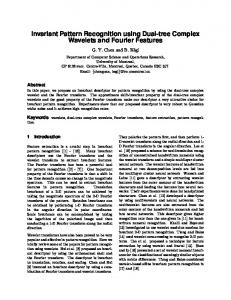
(b) F 0 (x) = F (x) + ²(x)
(a) F (x) = ln x sin(4x)
First−order autocorrelation of F(x)
First−order autocorrelation of F’
ACorr(lags)
ACorr(lags)
0
Lags
Lags
(c) First order autocorrealtion of F (x)
(d) First order autocorrelation of F 0 (x)
(e) Second order autocorrelation of F (x)
(f) Second order autocorrelation of F 0 (x)
Figure 1: First and second order autocorrelations of a function F (x) and of its noisy version F 0 (x). Note how the autocorrelations are less affected by the noise, than the original representation of the function.