Fachvorträge umerische Konzepte ExcerptVI: fromN the Proceedings of the COMSOL Users Conference 2006 Frankfurt
PDE-constrained Control Using COMSOL Multiphysics - Control of the Navier-Stokes Equations Thomas Slawig TU Berlin, Institut f. Mathematik, Strasse des 17. Juni 136 MA 4-5, 10623 Berlin, Germany,
[email protected].
Abstract We show how the numerical solution of control problems constrained by Partial Differential Equations (PDEs) can be computed using COMSOL Multiphysics and its scripting language. We present the method to derive the optimality system, i.e. the necessary conditions for a minimum, and show how to implement and solve it using COMSOL Multiphysics‘ built-in nonlinear damped Newton method. As example we use distributed and boundary control of the stationary incompressible Navier-Stokes equations (NSE). The same technique can be used for different state equations. Keywords Optimal control, Navier-Stokes equations, Finite element method
to rigid walls with a no-slip condition. • a part with Dirichlet boundary conditions for the velocity, when this is used as control. This refers to blowing/ sucking or applying a tangential force on the fluid. For distributed control we set this part to be empty. • a part with a natural boundary conditions. These are incorporated implicitly in the weak formulation, as we will show later. For the NSE this is a mixed condition for the outer normal derivative of the velocity and the pressure. This condition represents a free outflow region and is sometimes also referred to as a ‚‘do nothing‘‘ condition. Since COMSOL Multiphysics is a finite element package and also the technique to derive the optimality system we use below relies on weak formulations we present the corresponding one of the NSE her briefly.
1. Introduction: PDE-constrained Control Problems The general form of a PDE-constrained control problem is the following. The aim is to minimize a functional J=J(y,u) under the constraint of a PDE that is written in the form e(y,u)=0. Here y denotes the state, i.e. the solution of the PDE, and u the control. Clearly the state depends on the control, such that we have y=y(u). The state consists of field variables (for example the pair of velocity vector v and pressure p in a flow problem). The control can be either a distributed quantity, which results in a inhomogeneity of the PDE, or a function defined on the whole or parts of the boundary of the computational domain, thus affecting the boundary conditions.
2. The Navier-Stokes Equations The NSE describe the flow of an incompressible Newtonian fluid. Unknowns are velocity vector (v) and pressure (p). The stationary equations read
The brackets denote the inner product in L2, the space of square-integrable functions. We do not go into the details of the choice of appropriate spaces V and P which are rather standard, see e.g. [2]. Let us just note that the do nothing condition disappears if we choose the test space W in the weak form such that w=0 on the Dirichlet and control boundary, but with no restriction on w on the remaining part.
3. Adjoint Equation and Optimality System for the NSE We now show the general process to get the optimality system. We introduce the Lagrange functional associated with the constrained problem
min J(y,u) subject to e(y,u).
Note that we do not discuss the function spacing setting here which is necessary to make our technique sound. For details with this respect we refer to [1]. The Lagrangian is defined as The boundary conditions are formulated in a rather general way with
• a part with Dirichlet boundary conditions for the velocity. These may be inhomogeneous which refers to an prescribed in- or outflow, or homogeneous which refers
where z is the adjoint variable or Lagrange multiplier, and the brackets denote an appropriate inner product in the used function spaces.
COMSOL ANWENDERKONFERENZ 2006
L(y,u,z) := J(y,u) + (z,e(y,u))
Seite 181
Fachvorträge VI: N umerische konzepte Excerpt from the Proceedings of the COMSOL Users Conference 2006 Frankfurt Usually in the case of a PDE the constraint e(y,u)=0 actually consists of several equations. In this case z becomes a vector, and the inner product ocurring in the Lagrangian L is replaced by the sum of the inner products of the adjoint variables with the corresponding constraints. For the NSE we set y:=(v,p) and obtain (d+3) Lagrange multipliers where d is the space dimension. For convenience we denote the vector of the first d multipliers - that correspond to the constraint of the momentum balance of the NSE - by z. We just consider the case d=2 here, the 3-D case is straight-forward. Now the Lagrangian has the form
variables have been eliminated. This system is called optimality system. Note that the adjoint equation is always linear.
4. Implementing the Optimality System in COMSOL Multiphysics Script The NSE are already given in COMSOL Multiphysics as an application mode. Thus it is not necessary to implement them again in the scripting language. But since we want to solve the whole optimality system - including the adjoint equation - here in a one-shot approach, we have to either use two application modes in a multiphysics setting or to define the optimality system as a separate PDE. In this paper we present how to do the latter, also because it is rather simple to write the NSE in the script language. We use the general form where a PDE is written as
The mathematical theory now states (note again that we skip any analytical details here) that a solution to the constrained problem is a saddle point of the Lagrangian. The necessary optimality condition for a saddle point of L (and thus a candidate for a minimum of J under the PDE constraint) can now be computed by setting the partial derivatives of L with respect to y, u, and z equal to zero. Doing so we get three sets of equations. At first the so-called adjoint equation - by setting the partial derivative of L w.r.t y to zero. In our case it reads (after carefully making use of Green‘s formula):
By setting the partial derivative of L w.r.t u to zero we get a relation between adjoint variable z and control u:
The optimality system now consists of N=2(d+1)=6 equations, where the first group corresponds to the original NSE and the last to the adjoint equation:
We thus obtain
4.1 Boundary Conditions The boundary conditions on each boundary partition are written as
To define Dirichlet conditions G=0 is set. Then the first equation imposes no condition on the unknowns because of the free Lagrange multipliers mm. The second integral in the cost function J incorporating the control is called regularization term. The last necessary condition for a saddle point of the Lagrangian is the state equation itself - obtained by setting the partial derivative of L w.r.t z to zero. The representations of the controls can be inserted directly in the state equation, and together with the adjoint equation we obtain a coupled system from which the control Seite 182
By defining R the Dirichlet conditions are specified. For a boundary section with free outflow conditio R=0 is set. The Lagrange multipliers are now meaningless. We thus get for a problem where the Dirichlet boundary is split up into one partition with homogeneous conditions (corresponding to a wall) and another one with inhomogeneous conditions (region with a prescribed inflow function, here g) the following setting. For every boundary partition the first group of settings corresponds to the boundary conCOMSOL ANWENDERKONFERENZ 2006
Fachvorträge umerische Konzepte ExcerptVI: fromN the Proceedings of the COMSOL Users Conference 2006 Frankfurt ditions for the NSE, and the second group to those for the adjoint equation.
5. Control Using COMSOL Multiphysics via a One-shot Approach
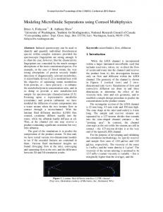
Figure 1. Streamlines (top), and ditribution of the cost (middle) for the uncopntrolled flow over a backward facing step flow).
In this section we show how a control problem for the stationary NSE can be solved with COMSOL Multiphysics. Following the idea to solve the whole optimality system and using the coupling information between adjoints and control leads to a rather short implementation. If the state equation is non-linear an appropriate solver is Newton‘s method. In every step of the newton iteration a linear system has to be solved. The one shot approach doubles the size of the whole system (compared to a solution of the state equations alone), and thus also of the linearized systems to be solved in each Newton step. A different approach solving the problem by an iterative scheme can be found in [4]. As numerical example we present a typical CFD test application, namely boundary control for a backward facing step channel flow. Free outflow conditions were imposed at the end of the channel, and a parabolic inflow was imposed on the inlet. For high values of the Reynolds number Re=1/n there is a long separation bubble behind the step. Aim was to reduce this bubble. For this purpose we used the cost functional
Figure 2. Streamlines (top), value of the cost (middle) and final control (bottom) for the controlled backward facing step flow,V alue of the cost is without regularization term.).
done here, we just set the minimum damping rate rather small. The Newton did not converge in all cases, still the obtained controls produced Results that significantly reduced the cost. The method was also applied to distributed control problems and also 3-D cases. Extensions to problems with additional constraints on the control variables are under investigation. References
which was also used in [3]. The velocity on the vertical wall of the step was used as control parameter, the Reynolds number was set to 1000. We started with a regularization parameter a=1 and used the soltuion as initial value for runs with a00.1, and so forth for a=0.01. The results are shown in Figures 1 and 2 below. As can be seen in the pictures below the optimization was quite successful using this. Further tuning of the solver was not
COMSOL ANWENDERKONFERENZ 2006
[1] T. Slawig: PDE-constrained Control Using FEMLAB - Control of the Navier-Stokes Equations, to appear in: Numerical Algorithms, online version available on www.springerlink. com (2006). [2] V. Girault, P.-A. Raviart: Finite Element Methods for Navier Stokes Equations, Springer Series in Comp. Math. 5, New York (1986). [3] M. Desai, K. Ito: Optimal controls of Navier-Stokes equations, SIAM J. Control Optimization 32(5), 1428-1446 (1994). [4] L. H. Olesen, F. Okkels, H. Bruus: A high-level programming-language implementation of topology optimization applied to steady-state Navier-Stokes flow, Int. J. Numer. Meth. Engng. 65, 975-1001 (2006).
Seite 183