Performance Comparison of Neural Networks and GMM for Vocal ...

Ananya Bonjyotsna et al. / International Journal of Engineering and Technology (IJET)

Performance Comparison of Neural Networks and GMM for Vocal/Nonvocal segmentation for Singer Identification Ananya Bonjyotsna #1, Manabendra Bhuyan #2 #

Dept of Electronics and Communication Engg, Tezpur University Assam, India 1 [email protected] 2 manab@ tezu.ernet.in

Abstract— Vocal and nonvocal segmentation is an important task in singing voice signal processing. Before identifying the singer it is necessary to locate the singer’s voice in a song. Maximum of the songs start with a piece of instrumental accompaniment known as ‘prelude’ in musical terms after which the singing voice comes into play. Therefore, it is necessary to detect the vocal region in the song in order to extract the singer’s voice characteristics and to avoid the non-vocal region which includes the instrumental accompaniment. This work thus classifies Vocal and Nonvocal region in songs using three different classifiers: Gaussian Mixture Model (GMM), Artificial Neural Network (ANN) with Feed Forward Backpropagation algorithm and Learning Vector Quantization (LVQ). Mel Frequency Cepstral Coefficient (MFCC) has been considered as the primary feature for classification. An available database MUSCONTENT is used and a newly created Database ASDB1 consisting of sixty excerpts from a wide variety of Assamese songs has been examined applying the same methods of classification. The efficacy of the classifiers has been tested and the results indicate that LVQ is a robust classifier compared to FFBP and GMM. Keywords-Music information Retrieval (MIR), Singer Identification (SID), Gaussian Mixture Model (GMM), Artificial Neural Network (LVQ and FFPB), Mel Frequency Cepstral Coefficient (MFCC). I. INTRODUCTION Music Information Retrieval (MIR) is a growing research area that intrigues people from both the research community and music industry. It deals with retrieving and querying of information from any music and exploits this information for real world problems such as Singer Identification, Music Categorization, Music Transcription, Music generation, instrument recognition etc [1]. Vigorous research has been going on over a decade in the field of Singer Identification. Extracting singing voice features appropriately is a challenging task since the singing voice is accompanied with background music. Singer Identification (SID) is the process of retrieving the identification of the singer in a song through features of the singer’s voice. Sensitivity to the human voice reception has evolved as an improvement of our auditory physiology and perceptual apparatus. Once we hear a person speaking, it is relatively easier to identify that voice with very little training. Similar is the case with regards to the singing voice. Once we become familiar with the sound of a particular singer’s voice, without much struggle we can usually identify the voice, even when hearing a song for the first time. One could subconsciously conjecture the singer when one hears a song. Therefore, all audio systems, the music stores and the online stores usually categorize music by the names of singers. For content-based Music Information Retrieval (MIR), it is necessary to extract the characteristic features of the particular singing voice. Hence, study based on using vocal segment in a song for retrieval is rather necessary. In singer identification location of vocal/nonvocal segment is an important pre-processing stage [2]. Therefore in this paper we provide a novel method of comparison of three different classifiers for vocal/nonvocal segmentation required for SID. II. A REVIEW Many different approaches have been made by different researchers to classify the vocal and nonvocal parts. Basically in most of these statistical classifiers modeling the vocal and nonvocal part separately has been applied. For classification of any signal two main components are required which are (1) features and (2) classifiers. Different features namely Mel-frequency Cepstral Coefficients (MFCC), Linear Predictive Coefficients (LPCs), Perceptual Linear Prediction Coefficients (PLPs) and the Harmonic Coefficients have been used for singing voice detection. Features like MFCC, LPC, and PLP are also widely used for general sound classification tasks and they are called short term features because they are calculated in short time frames. Similarly different classifiers have also been explored including Gaussian Mixture Models (GMM), Hidden Markov Model (HMM), Support Vector Machines (SVMs) and multilayer perceptrons (MLPs). Some researchers have also applied the direct energy distribution criteria and filtering to detect the vocal segment.

ISSN : 0975-4024

Vol 6 No 2 Apr-May 2014

1194

Ananya Bonjyotsna et al. / International Journal of Engineering and Technology (IJET)

Berenzweig and Ellis [3] used a speech recognizer’s classifier to distinguish vocal segments from accompaniment. They have used a neural network acoustic model for classification. They have used Posterior Probability Feature (PPF) as a feature. However, in this method it is found that PPF produced more errors than the cepstral coefficients. Tsai and Wang [4] constructed separate models for vocal and instrumental part using GMM and classified using log-likelihoods. They used MFCC as their feature and carried our frame wise classification. However, their technique fails to adapt to the human perception of hearing since frame switching was done within 0.5sec. Since majority of energy in the singing voice falls between 200Hz and 2000Hz, Kim and Whitman [5] has developed a straight forward method to detect energy within the frequencies bounded by the range of vocal energy. They have used a simple Chebychev infinite-impulse response (IIR) digital filter of order 12 to filter the audio signal and an Inverse Comb filter to filter out the frequency range of drums and their harmonics bandpassing the vocal range to pass through while attenuating other frequency regions. They have used thresholding technique to separate out the vocal part. However, it is difficult to choose a threshold value which requires a priori knowledge about the signal and therefore it may produce a false classification to a new tested singing voice. Nwe and Li [6] put forwarded a novel approach to extract the vocal segments. Firstly the vocal and nonvocal parts are trained using HMM models by manually annotated songs and then performed classification between vocal and nonvocal segments. They also developed adaptive HMM to adapt to the temporal changes in the song and as well provided with a hypothesis test to further validate the classification result. Multimodel HMM was introduced here for Nonvocal, Intro, Bridge, Chorus, Outro and developed three models λ v, λ I and λ CBO . Here the vocal-non vocal classification obtained is a maximum of 70.9% for CBO while 47.5% and 57.4% only for vocal and Intro. Li and Wang [7] have also performed classification with HMM taking Signal to Noise ratio as features. Nwe et al. [8] modified [7] specifying that different sections of a song (intro, verse, chorus, bridge, and outro) have different SNRs and they trained the classifier using wide range of SNRs and carried out 10-fold validation to check the overall performance. We therefore propose a novel and simple method of measuring the performance among the classifiers for vocal/nonvocal segmentation on two databases- MUSCONTENT and ASDB1. III.METHOD In this paper, experiments are carried out on an available database MUSCONTENT-PRACTICAL [9]. It is a database consisting of sixty 15-second excerpts from different English songs recorded at random by Scheirer and Slaney from radio and later on labelled by Berenzweig and Ellis. The same sets of analysis are also carried out on a newly created database of same length segments of Assamese songs named as ASDB1. This database also consists of sixty samples each of 15 seconds length. MATLAB tool is used as the platform to perform the experiments. The audio samples are in .WAV format. In order to classify the vocal from the nonvocal segments we need to first extract the characteristic feature of both the segments. Extraction of characteristic feature will provide us with the Feature Vectors which are then subjected to the classifier. The primary feature that is used here is the Mel Frequency cepstral Coefficient (MFCC). These coefficients form the Feature vectors which are fed to the classifiers. For classification we require both the training data and testing data. The Feature Vectors computed from the training data are trained for modelling in the training phase and in the testing phase the Feature Vectors of the test samples are matched with the trained models for classification. In this work, a statistical classifier GMM and knowledge based classifier ANN are used for classification. Two algorithms of ANN, Feed Forward Back Propagation and Learning Vector Quantization are implemented for this purpose. The segmentation process is showed in the block diagram in the Figure 1.

Fig 1: Vocal/Non-vocal segmentation.

ISSN : 0975-4024

Vol 6 No 2 Apr-May 2014

1195

Ananya Bonjyotsna et al. / International Journal of Engineering and Technology (IJET)

A. Mel Frequency Cepstral Coefficient The Cepstrum or cepstral coefficient, 𝐶(𝜏) is defined as the Inverse Fourier Transform (IFT) of the short-time logarithmic amplitude spectrum. The term cepstrum is a coined word which includes the meaning of the inverse fourier transform of the spectrum. The independent parameter for the cepstrum is called the quefrency. Since the cepstrum is the inverse transform of the frequency domain function, the quefrency becomes the time-domain parameter. The special feature of the cepstrum is that it allows for the separate representation of the spectral envelope and fine structure. MFCC is a traditional feature used for audio processing. The frequency bands in the Mel Filterbanks are equally spaced on the Mel-scale, which approximates the human auditory system's response more closely than the linearly-spaced frequency bands used in the normal cepstrum. Computation of MFCC involves the following steps [10]: 1) Pre-emphasis: Generally, Pre-emphasis is done on the input signal to balance the low and the high frequencies and to give equal weights. The original signal usually has too much lower frequency energy, and in order to emphasize the high frequency energy pre-emphasis is necessary. The signal is re-evaluated using the equation, Y[n] = x[n] - α x[n-1]

(1)

where α is the pre-emphasis coefficient and is considered to be 0.97. 2) Framing and windowing: The pre-emphasized signal is then divided into smaller frames of 25ms with a frame shift of 10ms. This is done because an audio signal is constantly changing, so to simplify it is assumed that on short time scales the audio signal doesn’t change much. Therefore a signal is optimally framed into 20-40ms. A Hamming window is applied to the frames which is given by the following equation: 𝑤(𝑛) = 0.54 − 0.46 cos �

2𝜋𝑛

𝑛−1

� 0≤𝑛 ≤𝑁−1

(2)

3) Fast Fourier Transform: The windowed signal is then subjected to Fourier Transform to obtain the power spectrum which is in frequency domain. The equation for finding the FFT is given below-

4)

−𝑗2𝜋𝑘𝑛/𝑁 𝑋(𝑘) = ∑𝑁−1 , 0≤𝑘 ≤𝑁−1 𝑛=0 𝑥(𝑛)𝑒

(3)

Filter Bank: Mel Filter Banks are applied to the FFT spectrum and then Inverse Transform is applied by DCT. In order to compute the Mel spaced filterbanks, the frequencies are converted to Mel scale by the formula given by 𝑀(𝑓) = 1125 ln (1 + 𝑓/700).

(4)

5) Discrete Cosine Transform The cepstral parameters are then calculated from the log filterbank amplitudes using the Discrete Cosine Transform using the following equation2

𝜋𝑖

𝐶𝑖 = � ∑𝑁 𝑗=1 𝑚𝑗 cos ( (𝑗 − 0.5)) 𝑁

𝑁

(5)

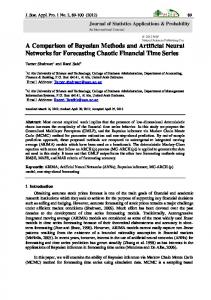
Where N is the Number of filter bank channels. The resulted coefficients are known as Cepstral Coefficients (CC). The set of coefficients is called Feature Vector. The block diagram for the computation of MFCCs is shown in the Figure 2. The Features extracted are then subjected to different machine learning techniques to build unique models for each singer or train each singer.

ISSN : 0975-4024

Vol 6 No 2 Apr-May 2014

1196

Ananya Bonjyotsna et al. / International Journal of Engineering and Technology (IJET)

Fig 2. Feature extraction of audio samples.

B. Gaussian Mixture Model GMM is one of the Bayesian classifiers that assumes a known probabilistic density distribution for each class. Data from each class is modeled as a group of Gaussian clusters. For d dimensions, the Gaussian distribution of a vector 𝑥 = (𝑥 1 , 𝑥 2 , … , 𝑥 𝑑 )𝑇 is defined by: 𝑁(𝑥|𝜇, Σ) =

1

(2𝜋)𝑑/2 �|Σ|

1

exp (− (𝑥 − 𝜇)𝑇 Σ−1 (𝑥 − 𝜇)) 2

(6)

Where µ is the mean and ∑ is the covariance matrix of the Gaussian distribution. The probability given in a mixture of K Gaussians is: 𝑝(𝑥) = ∑𝐾 𝑗=1 𝑤𝑗 . 𝑁(𝑥|𝜇𝑗 , Σ𝑗 )

(7)

Where 𝑤𝑗 is the prior probability (weight) of the jth Gaussian. The mixture weights have to satisfy ∑𝑘𝑗=1 𝑤𝑗 = 1

and 0≤𝑤𝑗 ≤1

The resulting parameters, mean vectors, covariance matrix and the weights from the training procedure represent the characteristic model of the singer. To obtain the parameters, the expectation maximization (EM) algorithm is used, which is an iterative implementation of maximum likelihood estimation. C. Feed forward Back Propagation Generally, a feedforward neural network is a combination of three layers of neurons: input layer, hidden layer and output layer. The neurons in these layers are activated by using an activation function. The backpropagation algorithm assumes feedforward neural network architecture. The number of input nodes is determined by the dimensionality of input patterns, and the number of nodes in the output layer is dictated by the problem under consideration. If it has to map a function of n-dimensional input vectors to m-dimensional output vectors, the network will contain n input nodes and m output nodes. The number of hidden layers is upto the discretion of the network designer and generally depends on the problem. The weights are updated in order to minimize the mean square error (MSE) between the predicted values and actual target values. In back propagation algorithm the weights and biases are modified as follows: W ij =W ij +δW ij

(8)

θ j= θ j +δ θ j

(9)

where, δθ j is change in bias and δW ij is change in weight. Gradient descent method is used to find set of weights that fits the training data to minimize the MSE. D. Learning Vector Quantization We have implemented LVQ2.1 algorithm in this work. This algorithm was developed by Kohonen. Learning vector quantization (LVQ), is a prototype-based supervised classification algorithm. It follows basically three steps for learning. First, if the input x and the associated weight W I(x) have the same class label, then move them closer together by the equation-

ISSN : 0975-4024

Vol 6 No 2 Apr-May 2014

1197

Ananya Bonjyotsna et al. / International Journal of Engineering and Technology (IJET)

∆𝑊𝐼(𝑥) (𝑡) = 𝛽(𝑡)(𝑥 − 𝑊𝐼(𝑥) (𝑡))

(10)

Secondly, if the input x and associated Voronoi vector/weight 𝑊𝐼(𝑥) have the different class labels, then move them apart by(11) ∆𝑊𝐼(𝑥) (𝑡) = −𝛽(𝑡)(𝑥 − 𝑊𝐼(𝑥) (𝑡))

where 𝛽(𝑡) is the learning rate. Lastly, the weights corresponding to other input regions are left unchanged with ∆wj(t) = 0. LVQ2 is a modified version of LVQ1 with certain additional conditions for updating the weights. IV. EXPERIMENTS At first MFCC coefficients are computed from the each audio file from the database MUSCONTENT. The audio files are in the .wav format. The sampling frequency of each of the audio file is 22.05KHz and each is 15seconds in length. The database consists of sixty labeled music excerpts some of which have vocals in it and some without the vocals. At the onset the audio files are manually annotated into vocal and nonvocal and shown below with the label numbers Music without Vocals=[1, 2 , 15, 16, 17, 18, 21, 23, 24, 32, 33, 34, 35, 38, 39, 40, 41, 42, 47, 49, 54, 55, 56, 57, 59]  Music with vocals=[3, 4, 5, 6, 7, 8, 9, 10, 11, 12, 13, 14, 19, 20, 22, 25, 26, 27, 28, 29, 30, 31, 36, 37, 43, 44, 45, 46, 48, 50, 51, 52, 53, 58, 60] For training, 10 files are considered out of which 5 files are taken from files which have voice in it and the other 5 consists of nonvocal music samples. Each audio file is framed at 25ms with 10ms overlapping. 26 numbers of mel filterbanks are computed and applied to the spectrum of the frames. Then the Inverse Transform is applied to the log of the filtered spectrum using DCT to get the cepstral coefficients. A matrix of the coefficients is evaluated from the file with each frame consisting of 13 MFCCs. These MFCCs form the feature Vector of that particular audio file. These 13 coefficients are fed to the input of the neural network. Two algorithms- feedforward backpropagation algorithm (FFBP) and Learning Vector Quantization (LVQ) is implemented for classification. Specifically these two algorithms are implemented because FFBP is a powerful supervised training algorithm which is used in varied applications and LVQ is based on straightforward approach to interpret data and also for its simpler neural network model. First, the data is separated into inputs and targets. The significant features extracted from the data act as the inputs to the neural network. The networks are simulated using MATLAB. A. Classification using FFBP and LVQ: For the FFBP, the targets for the neural network are indexed as integer 1 to denote presence of vocals and integer 0 for nonvocals in the FFBP. We have used an ANN structure as shown in Figure 3. The training parameters are set by trial and error to get the maximum training performance. Sigmoid transfer function is used for the hidden layer. Gradient descent backpropagation training function is used for training the weights. Number of epochs is set to 600 and learning rate of 0.5 is used. After fixing the parameters, training is performed on the training set which consists of 10 samples 1,2,15,16,17 from the vocals and 3,4,5,6,7 from the nonvocals. Testing is done on the rest of the samples. Frame wise training and validation is performed on the training set and shown in the table I. A 5-fold cross validation is performed for classification and Identification Accuracy (Id. Acc) for each fold is shown the Figure 7 and 8 in the results section. For LVQ, the targets are indexed as 1 for vocals and 2 for nonvocals, and the same set of training samples is used. The Frame accuracy result is shown in section V. A similar cross validation is performed which is provided in the results section. B. Classification using GMM. Matlab tool is used to implement GMM. Tests are performed taking different number of Gaussians for one class. In this case since five test samples are considered at a time, maximum of 5 Gaussians could be considered and full matrix of each component is taken for the covariance matrix. The results are presented in the next section. The same experiment for vocal/nonvocal classification is further carried out using a newly built database which consists of Assamese songs known as ASDB1. The sampling frequency of each file is 44.1KHz which is standard sampling frequency at present. For better comparison the number of audio files in the database is kept at 60. The files are labeled from 1 to 60 manually and divided into two parts viz vocals and nonvocals. While performing the experiment in ASDB1 the experimental parameters are kept unchanged as far as possible. Manually divided vocal/nonvocal samples are shown in the sets below and the results are presented in the next section.

ISSN : 0975-4024

Vol 6 No 2 Apr-May 2014

1198

Ananya Bonjyotsna et al. / International Journal of Engineering and Technology (IJET)



Music without Vocals = [ U1 U2 U6 U9 U11 U13 U16 U19 U20 U23 U25 U27 U29 U32 U35 U38 U40 U42 U44 U48 U49 U52 U45 U56 U57 U58]. Music with Vocals = [ V3 V4 V5 V7 V8 V10 V12 V14 V15 V17 V18 V21 V22 V24 V26 V28 V29 V30 V31 V33 V34 V36 V37 V39 V41 V43 V45 V46 V50 V51 V53 V54 V60 V47].



Fig 3: ANN structure for vocal/nonvocal classification.

V. RESULTS AND DISCUSSIONS The plot for two sample audio files is shown in the Figure 4 and Figure 5 with their respective spectra. (a) Waveform of a nonvocal music signal 1

Amplitude

0.5

0

-0.5

-1

0

5

10

15

Time(sec)

(b)

Single-Sided Amplitude Spectrum of y(t)

0.02

|Y(f)|

0.015

0.01

0.005

0

0

500

1000

1500

2000 2500 Frequency (Hz)

3000

3500

4000

4500

Fig 4: Nonvocal music signal. (a) Signal (b) Spectrum

ISSN : 0975-4024

Vol 6 No 2 Apr-May 2014

1199

Ananya Bonjyotsna et al. / International Journal of Engineering and Technology (IJET)

(a) Waveform of a vocal music signal 1

Amplitude

0.5

0

-0.5

-1

15

10

5

0

Time(sec)

(b)

Single-Sided Amplitude Spectrum of y(t)

0.02

|Y(f)|

0.015

0.01

0.005

0

500

0

3000

2500 2000 Frequency (Hz)

1500

1000

3500

4000

4500

Fig 5: Vocal music (a) Signal (b) spectrum

If we observe the two spectra carefully, we note that the vocal sample is rich in lower frequencies while in the non vocal spectrum the frequencies are more or less distributed equally. It also implies that the vocal region falls under the band of certain lower frequencies while the musical instruments have higher frequency components. This difference has been exploited by the reference [5] in their work. The respective MFCC cepstra of the signals above are also shown in the Figure 6. (a) Mel frequency cepstrum 12

15 10

Cepstrum index

8

10

6 5

4 0

2

-5 0 50

ISSN : 0975-4024

100

150

200

250 Frame index

300

Vol 6 No 2 Apr-May 2014

350

400

450

1200

Ananya Bonjyotsna et al. / International Journal of Engineering and Technology (IJET)

(b)

Mel frequency cepstrum 16

12

14 10 12

10 8

Cepstrum index

8

6

6

4 4 2

0

2

-2

0

-4 50

100

150

200

250 Frame index

300

350

400

450

Fig 6: MFCC (a) Nonvocal signal (b) Vocal signal

As we can see from the plots of MFCC the distinctive energy difference between the two signals, it is also evident that the zeroth order cepstral coefficients have higher energy associated with it in case of vocals and lesser energy in case of nonvocals. Although many researchers have pointed out the limitations of MFCC in the field of MIR, no one could possibly avoid using MFCC in their works. Hence it is understood without a doubt that MFCC still is a powerful feature when it comes to audio. Therefore in this work MFCC is used as a primary feature alone. Also this experiment is carried out for the case of binary classification i.e. an element can either belong to one group or the other which is the sole purpose of using only MFCC. These 13 coefficients extracted from the audio files are fed as inputs to the neural network using FFBP and LVQ which gives the frame wise classification results of the samples as shown in the table I and II respectively and the vocal/nonvocal classification accuracy for the 5-fold cross validation in Figure 7 and 8 respectively. TABLE I Frame-wise Classification Accuracy using FFBP

ISSN : 0975-4024

No. of Frames

Classification %

50 Frames

75

100 Frames

82

150 Frames

82

200 Frames

84

300 Frames

84

Vol 6 No 2 Apr-May 2014

1201

Ananya Bonjyotsna et al. / International Journal of Engineering and Technology (IJET)

90 80 70 60 50 40 30 20 10 0

76.67

73.33

68.33

First

Second

Third

81.67

85

Fourth

Fifth

Fig 7: Percentage Classification Accuracy using FFBP for 5-fold cross validation. TABLE II Frame-wise Classification Accuracy using LVQ

Frame

Classification(%)

50

75

100

75

150

75

200

80

300

80

Fig 8: Percentage Classification accuracy using LVQ for 5-fold cross validation

From Table I and II it is seen that considering 200 frames in both FFBP and LVQ give better classification accuracy. Therefore considering 200 frames for both the algorithms a 5-fold cross validation is performed. Figure 7 and Figure 8 shows the results of cross validation with their percentage accuracies. The average accuracy shown by FFBP is 77% and by LVQ is 77.6%. Now classifying using GMM also yields the results shown in Table III. Five samples each from vocal and non vocal are trained and GMM is tested with 5 different mixture models. The average result is considered from 1 Gaussian per class to 5 Gaussians per class.

ISSN : 0975-4024

Vol 6 No 2 Apr-May 2014

1202

Ananya Bonjyotsna et al. / International Journal of Engineering and Technology (IJET)

TABLE III Classification accuracy using GMM

Training set

Average Accuracy with different centres (%)

First Second Third Fourth Fifth

69.6 49.6 57.2 64.8 60

Average Accuracy with all cross validation (%)

60.24

From the experiment performed on MUSCONTENT it is deduced that neural networks performed better than GMM. Now when the same experiment is done on ASDB1, we get the following results presented in table IV. TABLE IV Classification accuracy for ASDB1

Training Set

First Second Third Fourth Fifth

5-fold cross validation Average acc (%) FFBP 65 63.33 61.67 54.4 43.33

LVQ 73.33 75 60 78.33 73.33

GMM 80.4 79.6 64.4 73.2 82

Average acc with all cross

validation (%) FFBP

LVQ

GMM

57.54

71.998

75.92

From the results shown in table IV, it is surprising to note that FFBP performed poorly whereas GMM showed improved classification accuracy. Therefore it is quite evident that FFBP and GMM are vulnerable to different databases and they may be dependent on the data. Importantly LVQ depicted consistency in performance in both the databases. VI. CONCLUDING REMARKS This work reveals the robustness of the LVQ algorithm in an application of binary classification i.e. vocal/nonvocal segmentation. A set of experiments are done on two databases MUSCONTENT and ASDB1 using three classifiers viz FFBP, LVQ and GMM. It is found that LVQ and FFBP showed better results of average classification accuracy of 77.6% and 77% respectively in the first database and GMM results an average accuracy of 60.24%. But in the second database, GMM has excelled in performance and FFBP showed poorer result whereas LVQ performed fairly. The average classification accuracies of FFBP, LVQ and GMM for the database ASDB1 are 57.54%, 71.99% and 75.92% respectively. FFBP and GMM are found to be showing contradictory results in two databases while LVQ has shown a relatively consistent accuracy in both the databases. Therefore LVQ has stood out as a better performer in comparison with FFBP and GMM with respect to binary classification of vocal and nonvocal regions. The percentage accuracy can be increased by addition of few more features along with MFCC which will lead to a better classifier for this application. The reason for showing contradictory results by the two classifiers is yet to be analyzed which gives enough scope for future work. REFERENCES [1] [2]

Fu, Z. A Survey of Audio-Based Music Classification and Annotation, IEEE transactions on multimedia, Vol. 13(2), 303-319,2011 Bonjyotsna, A.; Bhuyan, M., "Signal processing for segmentation of vocal and non-vocal regions in songs: A review," Signal Processing Image Processing & Pattern Recognition (ICSIPR), 2013 International Conference on , vol., no., pp.87,91, 7-8 Feb. 2013 [3] Berenzweig, A.L.; Ellis, D.P.W.; , "Locating singing voice segments within music signals," Applications of Signal Processing to Audio and Acoustics, 2001 IEEE Workshop on the , vol., no., pp.119-122,2001 [4] Wei-Ho Tsai; Hsin-Min Wang; , "Automatic singer recognition of popular music recordings via estimation and modeling of solo vocal signals," Audio, Speech, and Language Processing, IEEE Transactions on,vol.14,no.1,pp.330-341,Jan.2006 [5] Y.E.Kim and B.Whitman,”Singer identification in popular music recordings using voice coding features,” in Proc. 3rd Int. Conf. Music Inf. Retrieval (ISMIR 2002), 2002, pp. 164-169. [6] Nwe, T. L.; Li, H.; , "Exploring Vibrato-Motivated Acoustic Features for Singer Identification," Audio, Speech, and Language Processing, IEEE Transactions on , vol.15, no.2, pp.519-530, Feb. 2007 doi: 10.1109/TASL.2006.876756 [7] Yipeng Li; DeLiang Wang; "Separation of Singing Voice From Music Accompaniment for Monaural Recordings," Audio, Speech, and Language Processing, IEEE Transactions on , vol.15, no.4, pp.1475-1487 [8] T. L. Nwe, A. Shenoy, and Y. Wang, “Singing voice detection in popular music,” in Proc. 12th Annu. ACM Int. Conf. Multimedia, 2004, pp. 324–327. [9] Ellis [online Home page]. Available: http://www.ee.columbia.edu/~dpwe/muscontent/practical/. Last updated 2003. [10] L.R. Rabiner and R.W.Schafer, Digital Processing of Speech Signals, Prentics-Hall, Inc., New Jersey, 1978.

ISSN : 0975-4024

Vol 6 No 2 Apr-May 2014

1203