Performance Evaluation of Quantum Merging: Negative ... - CiteSeerX

Performance Evaluation of Quantum Merging: Negative Queue Length Hiroshi Toyoizumi ∗ [email protected] ∗

Waseda University Nishi-waseda 1-6-1, Shinjuku, Tokyo 169-8050 TEL: +81-3-3202-2293 FAX: +81-3-5286-1987

Abstract— We study the detail of queues handling quantum communication, especially socalled quantum merging of qubits. In quantum merging, by using EPR pairs (entangled pairs of quantum particles), jobs may bring extra service capacity to the server, which can be stored in the system for future use. We will model this phenomena as queues that can have the negative queue length, and show the basic characteristics of these quantum queues. Keywords: quantum merging, negative entropy, negative customer, queue, performance evaluation, virtual waiting time

1

Introduction

Quantum information processing is fundamentally different with its classical counterpart. The difference can be used to achieve something that classical information processing cannot achieve. For example, Shor’s algorithm[8] use qubits (quantum version of bits) to solve factorization problem effectively, which is notoriously hard to be solved by classical computers. This hardness is essential to the safety of RSA algorithm[7], that is used widely for secure communication on the internet. On the other hand, sometimes quantum information processing shows us something strange to interpret. One of those examples, is entropy. In classical Shannon’s theory, H(X), the entropy of a random variable X, is defined by X H(X) = − P {X = x} log P {X = x}. (1) x

The Shannon’s entropy measures the uncertainty of a data source, which is equivalent to how much information we can get when we learn the value of X. Suppose we have some partial data Y on our hand, which can be correlated with the source data X. Then, given Y , the amount of information we gained from X can be measured by the conditional entropy: H(X|Y ) = H(X, Y ) − H(Y ).

(2)

For example, if H(X|Y ) = 0, then X = f (Y ), which means we already have complete information of X. Thus, intuitively (and mathematically provable), H(X|Y ) is always nonnegative. In the quan-

tum world, the Neumann’s entropy S(ρ) and conditional entropy S(ρ|σ) are defined by S(ρ) = −tr(ρ log ρ),

(3)

S(ρ|σ) = S(ρ, σ) − S(σ),

(4)

for the density operators of quantum states ρ and σ. Although the Neumann’s entropy is a natural extension of Shannon’s entropy and measures the information carried, S(ρ) can be negative for EPR pairs (p.514 in [6]). In other words, we have the information more than certain for EPR pairs, which has been the mystery of quantum information theory. In 2005, Horodecki, Oppenheim and Andreas proposed the concept of partial information in [5]. They also introduced the framework called quantum merging to solve the mystery of negative quantum entropy. They showed that in the case when S(ρ) < 0, they can store the excess of the certainty in the bank and use them in the future. Thus, the performance of quantum merging is certainly different with the classical information processing. In this paper, we discuss the performance of the queue for quantum merging in detail, using queues that can have the negative queue length. In 1991, Gelenbe introduced the concept of negative customers in Markovian network setting[3]. There, a negative customers are supposed to erase one positive customer in queue while the queue length is positive. The stability and product form solution are studied in the papers like [3, 2, 11]. However, the negative customers in our model can be kept in the queue for the future use, even when there is no

positive customers. That is the main new concept derived from quantum merging.

2

Quantum Communication by Qubit Merging

We introduce the framework of quantum merging proposed in [5]. Suppose Alice wants to transfer the state of qubits to Bob. But in this case, Bob has his qubit, which is probably correlated with the state of Alice’s. In other words, Alice wants to send some information to Bob and merge her state to Bob’s. Let ρA and ρB be Alice and Bob’s density operator and let ρAB be the joint quantum state of Alice and Bob. Alice can use both the quantum channel and classical channel. Depending on the Bob’s quantum state, the procedure is different. Let us consider the following three cases. To distinguish the bits, we use |·iA for the Alice’s and |·iB for Bob’s bit.

Thus, it is clear that in quantum merging, the arrival of jobs (sending qubits) is not necessary a workload, but also enhance the service capacity, which is radically different from the classical bit merging.

3

Queues with Negative Queue Length

We model the quantum merging scheme and evaluate its performance using queueing theory. 3.1

Queuing Model and Negative Virtual Waiting Time

Suppose Alice and Bob build up a system for a quantum merging and open it for public. Customers arrive at the system carrying a qubit to merge to the receiver end. For the simplicity, we assume two types of customers:(1) whose qubit is independent with the receiver end, (2) whose qubit is entangled with the qubit at the receiver end. The first is called positive customers and the later is called 1. Independent states (S(ρA |ρB ) = 1). In this negative customers. The both positive and negative case, Alice has a random bit: customers arrive at the system with independent Poisson processes with the rate λp and λn , respec1 (5) ρA = (|0ih0|A + |1ih1|A ), tively. We can assume another type of customers 2 whose qubit is classically strongly-correlated. Howand Bob has his some state: ever, those customers doesn’t have to use quantum ρB = |0iB . (6) communication, so we ignore here. As showed in the Section 2, the positive customer The joint density matrix is has to send his state to the receiver with a quan1 tum channel, which is required some service time S. ρAB = (|0ih0|A + |1ih1|A )|0iB . (7) Maybe this will be done by using a photonic cable by 2 sending a new EPR pair. The service time S is asIn this case, Alice has to send one qubit with sumed to be independent and identically distributed the quantum channel to merge her state. with G(x) = P {S ≤ x}. On the other hand, a nega2. Classically strongly-correlated states (S(ρA |ρB ) = tive customer has a EPR pair, which can be used for 0). In this case the joint quantum state is sending the quantum state of a positive customer by using the quantum teleportation. We assume when1 ρAB = (|00ih00|AB + |11ih11|AB ). (8) ever there is a positive customer waiting, those EPR 2 pair of the negative customers will be used. When The mixed state can be considered a part of there is no positive customer in the system, we can pure state introducing a reference system R. save EPR pairs for future use. The queueing disThe state is already synchronized. Thus, Alcipline is assumed to be first-come-first-serve. Let ice doesn’t have to send any quantum inforN (t) be the number of customers in the system. We mation. Alice need to do some measurement allow N (t) to be negative. When the queue length (maybe for a reference system), then she can N (t) is negative, we have a pool of EPR pairs or use classical channel to send the result to Bob, negative customers in the system. The queue can then Bob can adjust his state locally to merge be called an M/G/1± queue for indicating to have Alice’s state. both positive and negative queue length. Here is the summary of the system transitions: 3. Entangled state (S(ρA |ρB ) = −1). The joint quantum state is a pure and entangled state, 1. When a positive customer sees N (t) < 0 at for example, his arrival, then he consumes one negative cus(9)

tomer to send his qubit and leaves the system immediately.

In this case, this EPR state is not only synchronized, but also has the ability to transfer other qubit (as a tool of quantum teleporation), while Bob creates a new EPR pair locally.

2. When a positive customer sees N (t) ≥ 0, then he joins the queue and waits for his service. His service will be terminated by the normal service completion required S, or by an arrival of negative customer.

1 |β00 i = √ (|00i + |11i). 2

3. When a negative customer sees N (t) > 0, then the customer in service finishes the service immediately and leave the system.

Vn(t)

positive arrival negative arrival

4. When a negative customer sees N (t) ≤ 0, then he will join the (negative) queue. t V(t)

positive arrival negative arrival positive departure

t

Figure 2: Vn (t): Virtual waiting time in the negatively censored process.

Figure 1: Virtual waiting time in a queue with negative queue length. Now we extend the definition of the virtual waiting time V (t) for the queues with negative queue length. Suppose an additional virtual positive customer has been arrived at our system at the time t. We allow this customer to arrive prior to the time t. The virtual waiting time V (t) is the difference between t and the time when this virtual customer starts his service. When the queue length is positive, the start time of his service is later than t, so V (t) is the same as the ordinary virtual waiting time. However, when the queue length is negative, this virtual customer could have started his service at the arrival of the negative customer who arrived earliest in the queue. Thus, V (t) can be both negative and positive. In Figure 1, we depict a sample path of our virtual waiting time process. We will evaluate the mean of the stationary version of the virtual waiting time E[V (t)] by censoring the virtual waiting time process. 3.2

Censoring and Idle-time Modification

In order to use ordinary queuing theory, we will break up our virtual waiting time process into pieces. Let us extend the notion of busy period in the case of V (t) < 0. Thus, when the system is idle, both negative and positive customers can start a new busy period. Since the positive and negative arrivals are Poisson process, the starts of new positive busy period are renewal points. We will pick only busy cycles started by negative customers and put them into one process (see Figure 2). Let Vn (t) be the virtual waiting time of this censored process.

it is easy to see that −Vn (t) is nothing but the attained sojourn time process. The attained sojourn time is probabilistically equivalent with the virtual waiting time, especially, the length of corresponding busy period length is the same [9]. Moreover, this negatively censored process has the same probabilistic structure with M/M/1 queues except the idle period. Note that idle periods are exponentially distributed with the mean 1/(λp + λn ), not 1/λn . Now we will modify the idle periods. We will take out all the idle period, then substitute them with new exponential random variables with the mean 1/λn , which is independent with others. Note that this modification will not affect the sample path of virtual waiting time in the busy period. The resulted modified process is an M/M/1 queue with the arrival rate λn and the service rate λp . Let Yn be the busy period of this modified process, then given λp > λn , we have E[Yn ] =

1 , λp − λn

(10)

(for example see [10, 4]). Further, let Wn (t) be the stationary version of the virtual waiting time of the modified process, then E[Wn (t)] =

λn /λp . λp − λn

(11)

By adjusting the idle period replacement, we can obtain the mean virtual waiting time of negative process, Vn (t) as E[Yn ] + 1/λn E[Wn (t)] E[Yn ] + 1/(λp + λn ) λn + λp . (12) = 2λp (λp − λn )

E[−Vn (t)] =

Now we consider the positive part. Just like the negative busy cycles, we will take out the positive

cycles and put them into one process. Let Vp (t) be the the virtual waiting time of this positive process. See Figure 3

of customers is assumed to be a Poisson process, we have Pp =

Vp(t)

(λp − λn )(µp + λn ) . (λp + λn )(µp − λn )

(17)

Also, Pn = 1 − Pp = t positive arrival negative arrival positive departure

Figure 3: Vp (t): Virtual waiting time in the positively censored process.

(18)

Note that these probabilities are insensitive with the second moment of the service time Sp . It is easy to see that the condition λp < µp will guarantee Pp < 1, since we have always µp = 1/E[min(S, Tn )] > λn . When the arrival rate of negative customers gets bigger and λn → λp , we have Pp → 0 and Pn → 1 as expected. On the other hand, when the arrival rate of positive customers approaches to the service rate µp , we have Pp → 1 and Pn → 0. 3.4

Next we modify all idle period with new exponential random variables with the mean 1/λp . The resulted modified process is an ordinary M/G/1 queue with the arrival rate λp and the i.i.d. service time Sp defined by

2λn (µp + λn ) . (λp + λn )(µp − λn )

Virtual Waiting Time

By conditioning on the busy cycle that a customer sees, we have E[V (t)] = E[V (t)|an arrival sees a positive cycle]Pp + E[V (t)|an arrival sees a negative cycle]Pn . (19)

Sp = min(S, Tn ),

(13)

where Tn is the time length to the next negative arrival and is the exponential random variable with its mean λn . Let µp = 1/E[Sp ], Yp be the length of busy period in this modified M/G/1 queue. Then, 1 E[Yp ] = . µp − λp

λp E[Sp2 ]/2 , 1 − λp /µp

(14)

(15)

3.3

(20)

E[V (t)|an arrival sees a negative cycle] = E[Vn (t)] λn + λp . (21) =− 2λp (λp − λn ) Hence, we have the mean virtual waiting time of this system: µ2p (λp − λn )E[Sp2 ]/2 (µp − λn )(µp − λp ) λn (µp − λp ) − . λp (µp − λn )(λp − λn )

E[V (t)] =

E[Yp ] + 1/λp E[Wp ] E[Yp ] + 1/(λp + λn )

(λp + λn )E[Sp2 ]/2 = . (1 + λn /µp )(1 + λp /µp )

(λp + λn )E[Sp2 ]/2 . (1 + λn /µp )(1 + λp /µp )

Similarly, by using (12)

by Pollaczek-Khinchine formula (see [10, 4]). Adjusting the replacement of the idle time, we have E[Vp (t)] =

E[V (t)|an arrival sees a positive cycle] = E[Vp (t)] =

Let Wp be the virtual waiting time of the modified M/G/1 queue, then given λp < µp , we have E[Wp ] =

Given that an arrival sees a positive cycle, V (t) is equivalent to Vp (t) in distribution. Thus, by using (16), we have

(16)

Busy Cycle that Arrivals See

Let Pp be the probability that a customer sees a positive busy cycle, and Pn be the probability that a customer sees a negative one. At the start of the busy period, a positive customer starts busy period with the probability λp /(λp + λn ). Since the arrival

(22)

Note that when we have no negative customers, λn = 0 and E[Sp2 ] = E[S 2 ] in (22). Thus, we have E[V (t)] =

λp E[S 2 ]/2 . 1 − λp E[S]

(23)

which is the usual Pollaczek-Khinchin formula for M/G/1 queues.

Let W be the the ordinary waiting time for customers in the stationary state. Note that negative customers always see no waiting time. Since the arrival is Poisson, W = max(V (t), 0) in distribution. Thus, E[W ] = E[Vp (t)]Pp

λp λp + λn

λp µ2p (λp − λn )E[Sp2 ]/2 = , (µp − λn )(µp − λp )(λp + λn )

(24)

where λn < λp < µp .

4

References [1] C Bennett, G Brassard, C Crepeau, R Jozsa, A Peres, and W Wootters. Teleporting an unknown quantum state via dual classical and EPR channels. Phys Rev Lett, pages 1895–1899, 1993. [2] P. Glynn E. Gelenbe and K. Sigmann. Queues with negative customers. Journal of Applied Probability, 28:245–250, 1991. [3] E. Gelenbe. Product-form queueing networks with negative and positive customers. Journal of Applied Probability, 28:656–663, 1991.

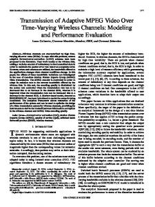
Example of an M/D/1± queue

[4] L. Kleinrock. Queueing Systems Vol. 1. John Wiley and Sons, 1975. 30% E!W" 5 70% 4 100%

3 2 1

1

0.5

1.5

2

Ρ

Figure 4: Mean waiting time in the M/D/1± queue. The percentage shows the ratio of positive customers in the arrival customers. The 100% corresponds to the ordinary M/D/1 queue. Let us consider an M/D/1± queue. The service time of customers S is constant, that is, S = 1/µ. In this case, 1/µp = E[Sp ] and E[Sp2 ] in (24) can be calculated by 1 E[Sp ] = E[min(S, Tn )] = {1 − e−λn /µ }. λn

(25)

2 2(µ + λn )e−λn /µ − . 2 λn λ2n µ

(26)

Figure 4 shows the mean waiting time of M/D/1± queues with S = 1. Unlike the ordinary M/D/1 queue, the mean waiting time will not blow up for ρ = λ/µ > 1. We can see “positive” effect of negative customers here.

5

[6] Isaac L. Chuang Michael A. Nielsen. Quantum Computation and Quantum Information. Cambridge Univ Pr, 2000. [7] R. L. Rivest, A. Shamir, and L. Adleman. A method for obtaining digital signatures and public-key cryptosystems. Commun. ACM, 26(1):96–99, 1983. [8] Peter W. Shor. Algorithms for quantum computation: Discrete logarithms and factoring. In IEEE Symposium on Foundations of Computer Science, pages 124–134, 1994. [9] Hiroshi Toyoizumi. Sengupta’s invariant relationship and its application to waiting time inference. J. Appl. Probab., 34(3):795–799, 1997. [10] R.W. Wolff. Stochastic modeling and the theory of queues. Princeton-Hall, 1989. [11] M. Miyazawa X. Chao and M. Pinedo. Queueing Networks, Customers, Signals and Product Form Solutions. John Wiley, 1999.

and E[Sp2 ] =

[5] Jonathan Oppenheim Micha Horodecki and Andreas Winter. Partial quantum information. Nature, 436:673–676, August 2005.

Conclusion

We develop a queueing model for quantum merging. The queueing model we proposed is the M/G/1± queue that can have the negative queue length and negative virtual waiting time. We derive the explicit form of the mean waiting time of as well as the mean virtual waiting time in this M/G/1± queue.